Page 339 - Fundamentals of Probability and Statistics for Engineers

322 Fundamentals of Probability and Statistics for Engineers

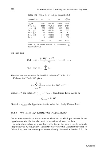
Table 10.3 Table for 2 test for Example 10.2
2
Interval, A i n i p i np i n /np i
i
x 0 5147 0.6188 4853 5459
0 < x 1 1859 0.2970 2329 1484
1 < x 2 595 0.0713 559 633
2 < x 3 167 0.0114 89 313
3 < x 4 54 0.0013 10 292
4 < x 5 14 0.0001 1 196
5 < x 6 0.0001 1 36
7842 1.0 7842 8413
Note: n i , observed number of occurrences; p i ,
theoretical P(A i ).

We thus have

0:48† i 1 0:48
e
P A i †ˆ p i ˆ ; i ˆ 1; 2; ... ; 6;
i 1†!
6
X
P A 7 †ˆ p 7 ˆ 1 p i ;
iˆ1
These values are indicated in the third column of Table 10.3.
Column 5 of Table 10.3 gives

k 2
X n
d ˆ i n ˆ 8413 7842 ˆ 571:
np i
iˆ1
With k ˆ 7, the value of 2 ˆ 2 is found from Table A.5 to be
:
k 1, 6, 0 01

:
2 ˆ 16 812:
:
;
6 0 01
Since d > 2 , the hypothesis is rejected at the 1% significance level.
6, 0: 01
10.2.2 THE CASE OF ESTIMATED PARAMETERS

Let us now consider a more common situation in which parameters in the
hypothesized distribution also need to be estimated from the data.
A natural procedure for a goodness-of-fit test in this case is first to estimate
the parameters by using one of the methods developed in Chapter 9 and then to
follow the 2 test for known parameters, already discussed in Section 7.2.1. In

TLFeBOOK