Page 344 - Fundamentals of Probability and Statistics for Engineers

Model Verification 327

10.3 KOLMOGOROV–SMIRNOV TEST

The so-called Kolmogorov–Smirnov goodness-of-fit test, referred to as the K±S
test in the rest of this chapter, is based on a statistic that measures the deviation

of the observed cumulative histogram from the hypothesized cumulative dis-

tribution function.
Given a set of sample values x 1 , x 2 ,.. . , x n observed from a population X, a
cumulative histogram can be constructed by (a) arranging the sample values in
increasing order of magnitude, denoted here by x (1) , x (2) ,..., x (n) , (b) determin-
ing the observed distribution function of X at x (1) , x (2) ,..., denoted by
0
0
0
F [x -1) ], F [x -2) ], . . . , from relations F [x -i) ] ˆ i/n, and (c) connecting the values
0
of F [x (i) ] by straight-line segments.
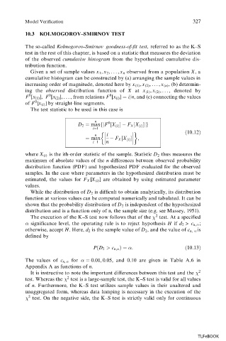
The test statistic to be used in this case is
n
0
D 2 ˆ maxfjF ‰X i† Š F X ‰X i† Šjg
iˆ1
10:12†

n i
ˆ max F X ‰X i† Š ;
iˆ1 n
where X (i) is the ith-order statistic of the sample. Statistic D 2 thus measures the
maximum of absolute values of the n differences between observed probability
distribution function (PDF) and hypothesized PDF evaluated for the observed
samples. In the case where parameters in the hypothesized distribution must be
estimated, the values for F X [X (i) ] are obtained by using estimated parameter
values.
While the distribution of D 2 is difficult to obtain analytically, its distribution
function at various values can be computed numerically and tabulated. It can be
shown that the probability distribution of D 2 is independent of the hypothesized
distribution and is a function only of n, the sample size (e.g. see Massey, 1951).
The execution of the K–S test now follows that of the 2 test. At a specified
significance level, the operating rule is to reject hypothesis H if d 2 > c n, ;

otherwise, accept H. Here, d 2 is the sample value of D 2 , and the value of c n, is
defined by
P D 2 > c n; † ˆ : 10:13†

:
The values of c n, for ˆ : 0 01, 0 05, and 0.10 are given in Table A.6 in
Appendix A as functions of n.
It is instructive to note the important differences between this test and the 2
test. Whereas the 2 test is a large-sample test, the K–S test is valid for all values
of n. Furthermore, the K–S test utilizes sample values in their unaltered and
unaggregated form, whereas data lumping is necessary in the execution of the
2 test. On the negative side, the K–S test is strictly valid only for continuous

TLFeBOOK