Page 338 - Fundamentals of Probability and Statistics for Engineers

Model Verification 321

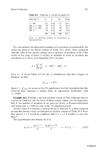
Table 10.2 Table for 2 test for Example 10.1
2
Interval, A i n i p i np i n /np i
i
t < 100 121 0.39 117 125.1
100 t < 200 78 0.24 72 84.5
200 t < 300 43 0.15 45 41.1
300 t 58 0.22 66 51.0
300 1.00 300 301.7
Note: n i , observed number of occurrences; p i ,
theoretical P(A i ).

For convenience, the theoretical numbers of occurrences as predicted by the
model are given in the fourth column of Table 10.2, which, when compared
with the value in the second column, give a measure of goodness of fit of the
2
model to the data. Column 5 (n /np i ) is included in order to facilitate the
i
calculation of d. Thus, from Equation (10.7) we have
k 2
X n
d ˆ i n ˆ 301:7 300 ˆ 1:7:
np i
iˆ1
Now, k ˆ 4. From Table A.5 for the 2 distribution with three degrees of
freedom, we find
2 ˆ 7:815:
3; 0:05

Since d < 2 , we accept at the 5% significance level the hypothesis that the
3, 0 05
:
observed data represent a sample from an exponential distribution with
ˆ 0 005.
.
Example 10.2. Problem: a six-year accident record of 7842 California drivers
is given in Table 8.2. On the basis of these sample values, test the hypothesis
that X, the number of accidents in six years per driver, is Poisson-distributed
with mean rate ˆ 0 08 per year at the 1% significance level.
.
Answer: since X is discrete, a natural choice of intervals A i is those centered
around the discrete values, as indicated in the first column of Table 10.3. Note
that interval x > 5 would be combined with 4 < x 5 if number n 7 were less
than 5.
The hypothesized distribution for X is

x 0:48
x t
t† e 0:48† e
p X x†ˆ ˆ ; x ˆ 0; 1; 2; .. . : 10:9†
x! x!

TLFeBOOK