Page 336 - Fundamentals of Probability and Statistics for Engineers

Model Verification 319

following Equation (10.6), random variable D thus approaches a chi-squared
distribution with one degree of freedom, and the proof is complete for k ˆ 2.
The proof for an arbitrary k proceeds in a similar fashion.
By means of Theorem 10.1, a test of hypothesis H considered above can be
constructed based on the assignment of a probability of Type-I error. Suppose

that we wish to achieve a Type-I error probability of . The 2 test suggests
that hypothesis H is rejected whenever
k 2
X n
d ˆ i n > 2 k 1; ; 10:7†
np i
iˆ1
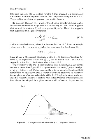
and is accepted otherwise, where d is the sample value of D based on sample
values x i , i 1, ..., n, andˆ 2 2 k 1, , takes the value such that (see Figure 10.1)

P D > 2 †ˆ :
k 1;
Since D has a Chi-squared distribution with (k 1) degrees of freedom for
large n, an approximate value for 2 can be found from Table A.5 in
k 1,
Appendix A for the 2 distribution when is specified.

The probability of a Type-I error is referred to as the significance level in this
context. As seen from Figure 10.1, it represents the area under f (d) to the right
D
of 2 . Letting ˆ :
0 05, for example, the criterion given by Equation (10.7)
k 1,
implies that we reject hypothesis H whenever deviation measure d as calculated
from a given set of sample values falls within the 5% region. In other words, we
expect to reject H about 5% of the time when in fact H is true. Which significance
level should be adopted in a given situation will, of course, depend on the

f D (d)

1– α

α
d
2
χ k–1, α
Figure 10.1 Chi-squared distribution with (k 1) degrees of freedom

TLFeBOOK