Page 71 - Fundamentals of Probability and Statistics for Engineers

54 Fundamentals of Probability and Statistics for Engineers

and
p ; for y ˆ 0;
8 5
>
>
> 4
> 5p q; for y ˆ 1;
>
>
> 3 2
<
X 10p q ; for y ˆ 2;
p y†ˆ p x i ; y†ˆ
Y XY 10p q ; for y ˆ 3;
2 3
i >
>
>
> 4
> 5pq ; for y ˆ 4;
>
>
: 5
q ; for y ˆ 5:
These are marginal pmfs of X and Y .
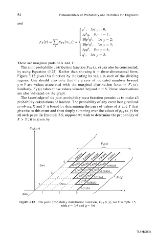
The joint probability distribution function F XY (x, y) can also be constructed,
by using Equation (3.22). Rather than showing it in three-dimensional form,
Figure 3.12 gives this function by indicating its value in each of the dividing
regions. One should also note that the arrays of indicated numbers beyond
y ˆ 5 are values associated with the marginal distribution function F X (x).
Similarly, F Y (y) takes those values situated beyond x ˆ 5. These observations
are also indicated on the graph.
The knowledge of the joint probability mass function permits us to make all
probability calculations of interest. The probability of any event being realized
involving X and Y is found by determining the pairs of values of X and Y that
give rise to this event and then simply summing over the values of p (x, y) for
XY
all such pairs. In Example 3.5, suppose we wish to determine the probability of
X > Y ; it is given by
F XY (x,y)
y
F (x)
X
0.07776 0.33696 0.68256 0.91296 0.98976
5 1
Zero 0.2592 0.6048 0.8352 0.9120 0.92224
0.3456 0.5760 0.6528 0.66304
3
0.2304 0.3072 0.31744 F Y (y)
0.0768 0.08920
1 Zero
0.01024
x
1 3 5
Zero
Figure 3.12 The joint probability distribution function, F XY (x,y), for Example 3.5,

with p ˆ 0:4 and q ˆ 0:6

TLFeBOOK