Page 72 - Fundamentals of Probability and Statistics for Engineers

Random Variables and Probability Distributions 55

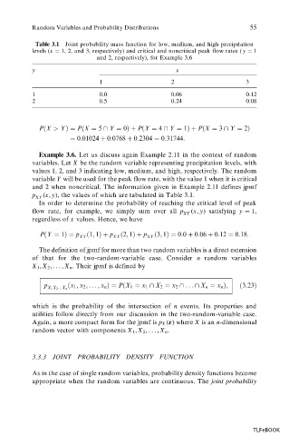
Table 3.1 Joint probability mass function for low, medium, and high precipitation
levels (x ˆ 1, 2, and 3, respectively) and critical and noncritical peak flow rates ( y ˆ 1
and 2, respectively), for Example 3.6
y x

1 2 3
1 0.0 0.06 0.12
2 0.5 0.24 0.08

P X > Y†ˆ P X ˆ 5 \ Y ˆ 0†‡ P X ˆ 4 \ Y ˆ 1†‡ P X ˆ 3 \ Y ˆ 2†
ˆ 0:01024 ‡ 0:0768 ‡ 0:2304 ˆ 0:31744:

Example 3.6. Let us discuss again Example 2.11 in the context of random
variables. Let X be the random variable representing precipitation levels, with
values 1, 2, and 3 indicating low, medium, and high, respectively. The random
variable Y will be used for the peak flow rate, with the value 1 when it is critical
and 2 when noncritical. The information given in Example 2.11 defines jpmf
p XY (x, y), the values of which are tabulated in Table 3.1.
In order to determine the probability of reaching the critical level of peak
flow rate, for example, we simply sum over all p XY (x, y) satisfying y ˆ 1,
regardless of x values. Hence, we have

P Y ˆ 1†ˆ p 1; 1†‡ p 2; 1†‡ p 3; 1†ˆ 0:0 ‡ 0:06 ‡ 0:12 ˆ 0:18:
XY XY XY
The definition of jpmf for more than two random variables is a direct extension
of that for the two-random-variable case. Consider n random variables
X 1 , X 2 ,..., X n . Their jpmf is defined by

p x 1 ; x 2 ; ... ; x n †ˆ P X 1 ˆ x 1 \ X 2 ˆ x 2 \ ... \ X n ˆ x n †; 3:23†
X 1 X 2 ...X n

which is the probability of the intersection of n events. Its properties and
utilities follow directly from our discussion in the two-random-variable case.
Again, a more compact form for the jpmf is p X (x) where X is an n-dimensional
random vector with components X 1 , X 2 ,... , X n .

3.3.3 JOINT PROBABILITY DENSITY FUNCTION

As in the case of single random variables, probability density functions become

appropriate when the random variables are continuous. The joint probability

TLFeBOOK