Page 74 - Fundamentals of Probability and Statistics for Engineers

Random Variables and Probability Distributions 57

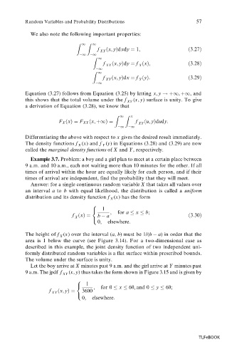
We also note the following important properties:
Z 1 Z 1
f x; y†dxdy ˆ 1; 3:27†
XY
1 1
1
Z
f x; y†dy ˆ f x†; 3:28†
XY X
1
1
Z
f x; y†dx ˆ f y†: 3:29†
XY Y
1
Equation (3.27) follows from Equation (3.25) by letting x, y !‡1, ‡1, and
this shows that the total volume under the f (x, y) surface is unity. To give
XY
a derivation of Equation (3.28), we know that
1 x
Z Z
F X x†ˆ F XY x; ‡1† ˆ f u; y†dudy:
XY
1 1
Differentiating the above with respect to x gives the desired result immediately.
The density functions f (x) and f (y) in Equations (3.28) and (3.29) are now
X
Y
called the marginal density functions of X and Y , respectively.
Example 3.7. Problem: a boy and a girl plan to meet at a certain place between
9 a.m. and 10 a.m., each not waiting more than 10 minutes for the other. If all
times of arrival within the hour are equally likely for each person, and if their
times of arrival are independent, find the probability that they will meet.
Answer: for a single continuous random variable X that takes all values over
an interval a to b with equal likelihood, the distribution is called a uniform
distribution and its density function f (x) has the form
X
1
8
< ; for a x b;
f x†ˆ b a 3:30†
X
0; elsewhere:
:
The height of f (x) over the interval (a, b) must be 1/(b a) in order that the
X
area is 1 below the curve (see Figure 3.14). For a two-dimensional case as
described in this example, the joint density function of two independent uni-
formly distributed random variables is a flat surface within prescribed bounds.
The volume under the surface is unity.
Let the boy arrive at X minutes past 9 a.m. and the girl arrive at Y minutes past
9 a.m. The jpdf f XY (x, y) thus takes the form shown in Figure 3.15 and is given by

1
8
< ; for 0 x 60; and 0 y 60;
f XY x; y†ˆ 3600
0; elsewhere:
:

TLFeBOOK