Page 165 - Fundamentals of Radar Signal Processing

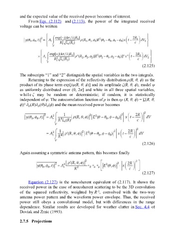
and the expected value of the received power becomes of interest.

From Eqs. (2.112) and (2.113), the power of the integrated received
voltage can be written

(2.125)

The subscripts “1” and “2” distinguish the spatial variables in the two integrals.
Returning to the expression of the reflectivity distribution ρ(R, θ, ϕ) as the
product of its phase term exp[jψ(R, θ, ϕ)] and its amplitude ζ(R, θ, ϕ), model ψ

as uniformly distributed over (0, 2π] and white in all three spatial variables,
while ζ may be random or deterministic; if random, it is statistically
independent of ψ. The autocorrelation function of ρ is then sρ (R, θ, ϕ) = |ζ(R, θ,
2
ϕ)| δ (R)δ (θ)δ (ϕ) and the mean received power becomes
D
D
D

(2.126)

Again assuming a symmetric antenna pattern, this becomes finally

(2.127)

Equation (2.127) is the noncoherent equivalent of (2.117). It shows the
received power in the case of noncoherent scattering to be the 3D convolution

of the squared reflectivity, weighted by R , convolved with the two-way
–2
antenna power pattern and the waveform power envelope. Thus, the received
power still obeys a convolutional model, but with differences in the range
dependence. Similar results are developed for weather clutter in Sec. 4.4 of
Doviak and Zrnic (1993).

2.7.5 Projections