Page 273 - Fundamentals of Radar Signal Processing

similar to the simple pulse, but with a good deal more tedium. An easier way is

to introduce the “chirp property” of the ambiguity function and then apply it to
the LFM case. Suppose that a waveform x(t) has an ambiguity function A(t, F ).
D
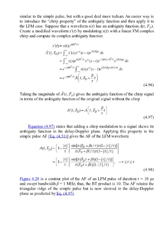
Create a modified waveform x′(t) by modulating x(t) with a linear FM complex
chirp and compute its complex ambiguity function

(4.96)

Taking the magnitude of Â′(t, F ) gives the ambiguity function of the chirp signal
D
in terms of the ambiguity function of the original signal without the chirp

(4.97)

Equation (4.97) states that adding a chirp modulation to a signal skews its
ambiguity function in the delay-Doppler plane. Applying this property to the
simple pulse AF [Eq. (4.51)] gives the AF of the LFM waveform

(4.98)

Figure 4.28 is a contour plot of the AF of an LFM pulse of duration τ = 10 μs
and swept bandwidth β = 1 MHz; thus, the BT product is 10. The AF retains the
triangular ridge of the simple pulse but is now skewed in the delay-Doppler
plane as predicted by Eq. (4.97).