Page 360 - Fundamentals of Radar Signal Processing

of the autocorrelation function of the clutter and the MTI filter impulse response

(Levanon, 1988; Nathanson, 1991). For low-order filters such as two- or three-
pulse cancellers and clutter power spectra with either measured or analytically
derivable autocorrelation functions, the resulting equations can be easier to
evaluate than the frequency domain versions.
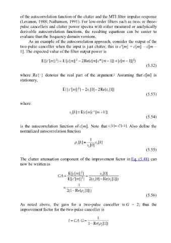
As an example of the autocorrelation approach, consider the output of the
two-pulse canceller when the input is just clutter; this is c′[m] = c[m] – c[m –

1]. The expected value of the filter output power is

(5.52)

6
where Re{·} denotes the real part of the argument. Assuming that c[m] is
stationary,

(5.53)

where

(5.54)

is the autocorrelation function of c[m]. Note that . Also define the
normalized autocorrelation function

(5.55)

The clutter attenuation component of the improvement factor in Eq. (5.48) can
now be written as

(5.56)

As noted above, the gain for a two-pulse canceller is G = 2; thus the
improvement factor for the two-pulse canceller is