Page 417 - Fundamentals of Radar Signal Processing

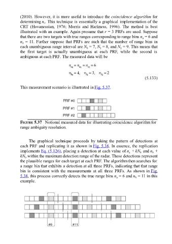
(2010). However, it is more useful to introduce the coincidence algorithm for

determining n . This technique is essentially a graphical implementation of the
t
CRT (Hovanessian, 1976; Morris and Harkness, 1996). The method is best
illustrated with an example. Again presume that r = 3 PRFs are used. Suppose
that there are two targets with true ranges corresponding to range bins n = 6 and
a
n = 11. Further suppose that PRFs are such that the number of range bins in
b
each unambiguous range interval are N = 7, N = 8, and N = 9. This means that
2
1
0
the first target is actually unambiguous at each PRF, while the second is
ambiguous at each PRF. The measured data will be

(5.133)

This measurement scenario is illustrated in Fig. 5.37.

FIGURE 5.37 Notional measured data for illustrating coincidence algorithm for
range ambiguity resolution.

The graphical technique proceeds by taking the pattern of detections at
each PRF and replicating it as shown in Fig. 5.38. In essence, the replication
implements Eq. (5.126), placing a detection at each value of n + kN and n +
a
b
0
kN within the maximum detection range of the radar. These detections represent
0
the plausible ranges for each target at each PRF. The algorithm then searches for
a range bin that exhibits a detection at all three PRFs, indicating that that range
bin is consistent with the measurements at all three PRFs. As shown in Fig.
5.38, this process correctly detects the true range bins n = 6 and n = 11 in this
a
b
example.