Page 257 - Fundamentals of Reservoir Engineering

OILWELL TESTING 194

p*
equ. (7.48) t n mlog t n
t
equ. (7.56) p*

p* t
sss mlog
p ws t
p sss

A B C
m m m

log t n log t
t t sss

4 3 2 1 0

log t + ∆t
∆t

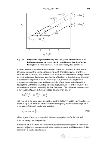
Fig. 7.20 Analysis of a single set of buildup data using three different values of the
flowing time to draw the Horner plot. A - actual flowing time; B - effective
flowing time; C - time required to reach semi-steady state conditions

It should be noted that the difference between plots A and B is not the same as the
difference between the buildups shown in fig. 7.19. The latter diagram is for three
separate sets of data, p ws as a function of ∆t, obtained in three different surveys. These
curves are displaced downwards as a function of the flowing time, that is, as a function
of the reservoir depletion. What is shown in fig. 7.20, however, is a single set of
pressure-time data interpreted as Horner plots for different assumed values of the
flowing time. Both the linear, extrapolated buildups, equs. (7.56) and (7.48), have the
same slope m, which is dictated by the final flow rate q n. The difference between them
is that a value of p ws on plot A is displaced laterally by an amount

t +∆ t t +∆ t t
log n − log ≈ log n
t ∆ t ∆ t

with respect to the same value on plot B, providing that both t and t n>>∆t. Therefore, as
shown in fig. 7.20, there is a vertical difference m log (t n/t) between the buildups for a
given value of ∆t which can be interpreted as

* * t
p − p = m log n (7.57)
n t t
*
*
where p and p are the extrapolated values of p ws(LIN) at ∆t = ∞ for the real and
n t
effective flowing time, respectively.
In addition, if it is assumed for a routine survey that the final flow period is sufficiently
long so that flow is under semi-steady state conditions, then the MBH equation, (7.44),
from which p can be calculated, is