Page 261 - Fundamentals of Reservoir Engineering

OILWELL TESTING 198

or

( p − p )
*
t +∆ t
log s = (7.62)
t ∆ s m

This equation, in which m = 162.6 q µ B o/kh, the slope of the buildup, demonstrates the
equivalence between the Dietz and MBH methods, which is also illustrated in fig. 7.21.

In particular, Dietz concentrated on buildup analysis for wells which were producing
under semi-steady state conditions at the time of survey, in which case, applying
equ (7.44), in field units

p D(MBH) = 2.303 log (C A t DA)

and therefore

t +∆ t
log s = log (C t ) (7.63)
ADA
t ∆
s
t +∆ t
from which the value of log s at which to enter the Horner plot can be calculated.
t ∆ s

An extension of Dietz method to determine pis frequently used in comparing observed
well pressures with average grid block pressures calculated by numerical simulation
models.

Physical no-flow
boundary

Grid block
boundaries in the
numerical simulation
A

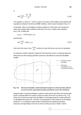
Fig. 7.22 Numerical simulation model showing the physical no-flow boundary drained
by well A and the superimposed square grid blocks used in the simulation

Suppose that a numerical simulation model is constructed so that there are several grid
blocks contained within the natural no-flow boundary of the well, as shown in fig. 7.22.
At the end of each time step in the simulation, the average pressure in each grid block
is calculated and printed out. Therefore, by interpolation in time between the simulated
pressures, it is a relatively simple matter to determine the individual grid block
pressures corresponding to the time at which a buildup survey is made in well A,