Page 329 - Fundamentals of Reservoir Engineering

REAL GAS FLOW: GAS WELL TESTING 264

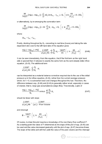
kh n Q 2 (t ) Q 1 ln 4A S DQ
−
i
1422T (m(p ) m(p wf n ) ) = ∆ j π DA n t − DA j 1 + n 2 γ C r 2 + + n
−
j1
Aw
=
or alternatively, by re-arranging the summation term
kh n t Q 1 ln 4A S DQ
−
i
j
1422T (m(p ) m(p wf n ) ) = 2π Q ∆ DA j + n 2 γ C r 2 + + n

j1
Aw
=
where
t ∆ DA j = t DA j − t DA j 1
−
Finally, dividing throughout by Q n, converting to real time (hours) and taking the rate
dependent skin over to the left hand side of the equation gives

m(p ) m(p wf n ) FQ 2 n 2.359T n Q j 1422T 1 ln 4A S (8.46)
−
−
i
j
j1 Q
( ) c Ah
Q n = φµ i n t ∆ + kh 2 γ C r 2 +
A w
=
It can be seen immediately, from this equation, that if the first term on the right hand
side is ignored then it reduces to exactly the same form as the semi-steady state inflow
equation, (8.43). The additional term
n
2.539T Q j t ∆
( ) cAh
φµ j1 Q j
i = n
can be interpreted as a material balance correction required due to the use of the initial
pressure p i in the inflow equation, (8.43), rather than the current average pressure
which, for t > 0, is somewhat lower and changes throughout the test. Therefore, the
difference between equ. (8.46) and (8.43) is generally rather small, especially in cases
of interest, that is, large gas accumulations (large Ahφ). Theoretically, a plot of

m(p ) m(p wf n ) FQ 2 n n Q j
−
−
i
j1 Q
Q n versus n t ∆ j (8.47)
=
should be linear with slope
2.359T 2.359T
=
( ) c Ah
µ
φµ ( ) c × Pore Volume
i i
and intercept
1422T 4A
B = 1 2 ln + S
kh γ C r 2
Aw
Of course, to draw this plot requires a knowledge of the non-Darcy flow coefficient F.
As a starting point the value of F determined as the slope of the plot of equ. (8.45) can
be used and the value decreased gradually until the plot of equ. (8.47) becomes linear.
The slope of the latter plot will then yield the value of the pore volume and the intercept