Page 373 - Fundamentals of Reservoir Engineering

NATURAL WATER INFLUX 308

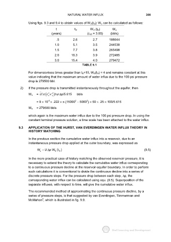
Using figs. 9.3 and 9.4 to obtain values of W D(t D); W e can be calculated as follows:

t t D W D (t D) W e
(years) (r eD = 3.00) (bbls)
.5 2.6 2.7 188644

1.0 5.1 3.5 244538
1.5 7.7 3.8 265498
2.0 10.3 3.9 272485
3.0 15.4 4.0 279472

TABLE 9.1

For dimensionless times greater than t D=15, W D(t D) = 4 and remains constant at this
value indicating that the maximum amount of water influx due to the 100 psi pressure
drop is 279500 bbl.

2) If the pressure drop is transmitted instantaneously throughout the aquifer, then
r -r
W e = cf π ( e 2 2 o ) hφ ∆p/5.615 bbls
2
-6
2
= 9 × 10 × .222 × π (15000 − 5000 ) × 50 × .25 × 100/5.615
W e = 279500 bbls

which again is the maximum water influx due to the 100 psi pressure drop. In using the
constant terminal pressure solution, a time scale has been attached to the water influx.

9.3 APPLICATION OF THE HURST, VAN EVERDINGEN WATER INFLUX THEORY IN
HISTORY MATCHING

In the previous section the cumulative water influx into a reservoir, due to an
instantaneous pressure drop applied at the outer boundary, was expressed as

()
W = U p W t D (9.5)
∆
D
e
In the more practical case of history matching the observed reservoir pressure, it is
necessary to extend the theory to calculate the cumulative water influx corresponding
to a continuous pressure decline at the reservoir-aquifer boundary. In order to perform
such calculations it is conventional to divide the continuous decline into a series of
discrete pressure steps. For the pressure drop between each step, ∆p, the
corresponding water influx can be calculated using equ. (9.5). Superposition of the
separate influxes, with respect to time, will give the cumulative water influx.

The recommended method of approximating the continuous pressure decline, by a
series of pressure steps, is that suggested by van Everdingen, Timmerman and
3
McMahon , which is illustrated in fig. 9.9.