Page 380 - Fundamentals of Reservoir Engineering

NATURAL WATER INFLUX 315

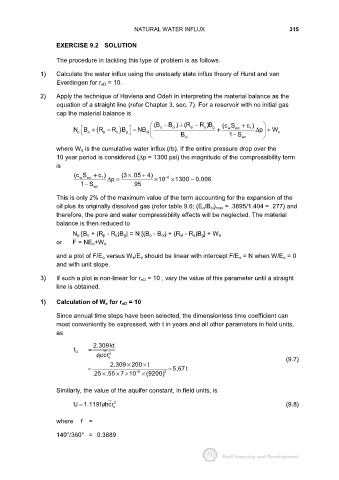
EXERCISE 9.2 SOLUTION

The procedure in tackling this type of problem is as follows.

1) Calculate the water influx using the unsteady state influx theory of Hurst and van
Everdingen for r eD = 10.

2) Apply the technique of Havlena and Odeh in interpreting the material balance as the
equation of a straight line (refer Chapter 3, sec. 7). For a reservoir with no initial gas
cap the material balance is

(B − B ) (R − R )B g (c S + c )
+
o
oi
si

s

NB + (R − R s )B = NB oi + w wc f ∆ p + W e

o
p
p
g
−
B oi 1 S wc
where W e is the cumulative water influx (rb). If the entire pressure drop over the
10 year period is considered (∆p = 1300 psi) the magnitude of the compressibility term
is
(c S wc + c ) p (3 .05 + 4) − 6 0.006
×
w
f
1S wc ∆= .95 × 10 × 1300 ∼
−
This is only 2% of the maximum value of the term accounting for the expansion of the
oil plus its originally dissolved gas (refer table 9.6; (E o/B oi) max = .3895/1.404 = .277) and
therefore, the pore and water compressibility effects will be neglected. The material
balance is then reduced to
N p [B o + (R p - R s)B g] = N [(B o - B oi) + (R si - R s)B g] + W e
or F = NE o+W e
and a plot of F/E o versus W e/E o should be linear with intercept F/E o = N when W/E o = 0
and with unit slope.
3) If such a plot is non-linear for r eD = 10 , vary the value of this parameter until a straight
line is obtained.

1) Calculation of W e for r eD = 10

Since annual time steps have been selected, the dimensionless time coefficient can
most conveniently be expressed, with t in years and all other parameters in field units,
as

2.309kt
t D =
φµ cr o 2 (9.7)
2.309 200 t
×
×
= = 5.67 t
6
−
× ×
×
.25.55 710 × (9200) 2
Similarly, the value of the aquifer constant, in field units, is
U1.119f hcr o 2 (9.8)
=
φ
where f =
140°/360° = 0.3889