Page 102 - Fundamentals of The Finite Element Method for Heat and Fluid Flow

94
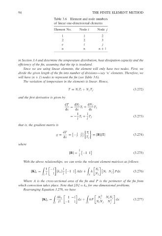
Table 3.6 Element and node numbers
of linear one-dimensional elements
Node j
Element No. Node i THE FINITE ELEMENT METHOD
1 1 2
2 2 3
e i j
n n n + 1

in Section 3.4 and determine the temperature distribution, heat dissipation capacity and the
efficiency of the fin, assuming that the tip is insulated.
Since we are using linear elements, the element will only have two nodes. First, we
divide the given length of the fin into number of divisions—say ‘n’ elements. Therefore, we
will have (n + 1) nodes to represent the fin (see Table 3.6).
The variation of temperature in the elements is linear. Hence,

T = N i T i + N j T j (3.272)

and the first derivative is given by
dT dN i dN j
= T i + T j
dx dx dx
1 1
=− T i + T j (3.273)
l l
that is, the gradient matrix is

dT T i

g = = − 1 l 1 l = [B]{T} (3.274)
dx T j
where

1
[B] = −11 (3.275)
l
With the above relationships, we can write the relevant element matrices as follows:

1 −1 1 N i

[K] e = [k x ] −11 Adx + h N i N j P dx (3.276)
l l 1 l S N j
Where A is the cross-sectional area of the fin and P is the perimeter of the fin from
which convection takes place. Note that [D] = k x for one-dimensional problems.
Rearranging Equation 3.276, we have

2
Ak x 1 −1 N i N i N j
[K] e = dx + hP 2 dx (3.277)
l l 2 −1 1 l N i N j N j