Page 101 - Fundamentals of The Finite Element Method for Heat and Fluid Flow

93
THE FINITE ELEMENT METHOD
(polynomials used) within an element remain unchanged under a linear transformation
from one Cartesian coordinate system to another. Polynomials that exhibit this invariance
property are said to possess ‘Geometric Isotropy’. Clearly, we cannot expect a realistic
approximation if our field variable representation changes with respect to a movement in
origin, or in the orientation of the coordinate system. Hence, the need to ensure geometric
isotropy in our polynomial interpolation functions is apparent. Fortunately, we have two
simple guidelines that allow us to construct polynomial series with geometric isotropy.
These are as follows:
(i) Polynomials of order ‘n’ that are complete, that is, those that contain all terms have
geometric isotropy. The triangle family satisfies this condition whether it be a linear,
quadratic or cubic form.
(ii) Polynomials of order ‘n’ that are incomplete yet contain the appropriate terms to
preserve ‘symmetry’ have geometric isotropy. We neglect only these terms that occur
3
2
2
3
in symmetric pairs that is, (x ,y ), (x y, xy ), and so on.
Example: For an eight-node element, the following polynomial, P , satisfies geometric
isotropy, that is,
2
P (x, y) = α 1 + α 2 x + α 3 y + α 4 x + α 5 xy + α 6 y 2 (3.269)
with either
3
α 7 x + α 8 y 3 (3.270)
or
2
2
α 7 x y + α 8 y x (3.271)
added to it.

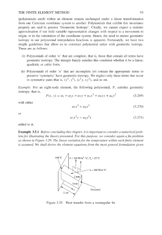
Example 3.5.1 Before concluding this chapter, it is important to consider a numerical prob-
lem for illustrating the theory presented. For this purpose, we consider again a fin problem
as shown in Figure 3.29. The linear variation for the temperature within each finite element
is assumed. We shall derive the element equations from the most general formulation given

100°C h = 120 W/m °C; T a = 25°C
2

k = 200 W/m°C
2mm

3mm
x Insulated
2 cm

Figure 3.29 Heat transfer from a rectangular fin