Page 103 - Fundamentals of The Finite Element Method for Heat and Fluid Flow

THE FINITE ELEMENT METHOD
Here N i = L i and N j = L j , which is generally true for all linear elements. Hence, we
can make use of the formula
95
a b a!b!l
L L dl = (3.278)
i
j
l (a + b + 1)!
For example,
2!0!l l
2 2
N dl = L dl = = (3.279)
i
i
l l (2 + 0 + 1)! 3
and other terms can be similarly integrated.
If A, k x ,P and h are all assumed to be constant throughout the element (see Figure 3.29),
we obtain the following [K] matrix:

Ak x 1 −1 hP l 21
[K] e = + (3.280)
l −1 1 6 12
Let us next consider the thermal loading. From Equation 3.261, we can write

GAl 1 qP l 1 hT a Pl 1
{f} e = − + (3.281)
2 1 2 1 2 1
In this case, the loads are distributed equally between the two nodes, which is a general
characteristic of linear elements.
The solution of the given problem may be found by substitution of the numerical values.
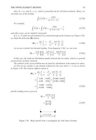
(a) First let us consider a one-element solution for the case where l = 2 cm, as shown
in Figure 3.30. The element stiffness matrix is

Ak x 1 −1 hP l 21
[K] e = +
l −1 1 6 12

0.06 −0.06 0.008 0.004
= +
−0.06 0.06 0.004 0.008

0.068 −0.056
= (3.282)
−0.056 0.068
and the loading term is given by

hP lT a 1
{f}=
2 1

0.30
= (3.283)
0.30
1 2

L = l = 2 cm

Figure 3.30 Heat transfer from a rectangular fin. One linear element