Page 106 - Fundamentals of The Finite Element Method for Heat and Fluid Flow

THE FINITE ELEMENT METHOD
98
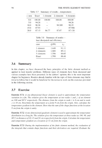
Table 3.7
x mm Exact Summary of results—temperatures
4 elements
1 element
2 elements
0.0 100.00 100.00 100.00 100.00
5.0 94.28 – – 94.26
10.0 90.28 – 90.209 90.25
15.0 87.93 – – 87.908
20.0 87.15 86.77 87.07 87.128
Table 3.8 Summary of results—
heat dissipated and efficiency
case Q(W) η f
1 element 1.640 91.11
2 elements 1.604 89.11
4 elements 1.596 88.65
Exact 1.590 88.48

3.6 Summary

In this chapter, we have discussed the basic principles of the finite element method as
applied to heat transfer problems. Different types of elements have been discussed and
various examples have been presented. In the authors’ opinion, this is the most important
chapter for beginners. Readers already familiar with the topic of finite elements may find it
trivial to follow but it would be beneficial for the novice to work out the exercises provided
in the following section.

3.7 Exercise

Exercise 3.7.1 A one-dimensional linear element is used to approximate the temperature
variation in a fin. The solution gives the temperature at two nodes i and j of an element
as 100 and 80 C respectively. The distance from the origin to node i is 6 cm and to node
◦
j is 10 cm. Determine the temperature at a point 9 cm from the origin. Also, calculate the
temperature gradient in the element. Show that the sum of the shape functions at the location
9 cm from the origin is unity.
Exercise 3.7.2 A one-dimensional quadratic element is used to approximate the temperature
distribution in a long fin. The solution gives the temperature at three nodes as 100, 90, and
◦
80 C at distances of 10, 15 and 20 cm respectively from the origin. Calculate the temperature
and temperature gradient at a location of 12 cm from the origin.

Exercise 3.7.3 During the implementation of the finite element method, the evaluation of
the integrals that contain shape functions and their derivatives are required. Evaluate the