Page 111 - Fundamentals of The Finite Element Method for Heat and Fluid Flow

STEADY STATE HEAT CONDUCTION IN ONE DIMENSION

k 103
T 1 T 2

x = 0 x = L
L
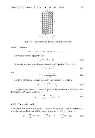
Figure 4.1 Heat conduction through a homogeneous wall

boundary conditions:

At x = 0,T = T 1 ; and at x = L, T = T 2
The exact solution to Equation 4.1 is

kAT = C 1 x + C 2 (4.2)
On applying the appropriate boundary conditions to Equation 4.3, we obtain

(4.3)
C 2 = kAT 1
and
kA(T 1 − T 2 )
C 1 =− (4.4)
L
Therefore, substituting constants C 1 and C 2 into Equation 4.3 results in
(T 1 − T 2 )
T =− x + T 1 (4.5)
L
The above equation indicates that the temperature distribution within the wall is linear.
The heat flow, Q, can be written as
dT kA
Q =−kA =− (T 2 − T 1 ) (4.6)
dx L

4.2.2 Composite wall
Even if more than one material is used to construct the plane wall, as shown in Figure 4.2,
at steady state, the heat flow will be constant (conservation of energy), that is,
k 1 A k 2 A k 3 A
Q =− (T 2 − T 1 ) =− (T 3 − T 2 ) =− (T 4 − T 3 ) (4.7)
x 1 x 2 x 3