Page 112 - Fundamentals of The Finite Element Method for Heat and Fluid Flow

STEADY STATE HEAT CONDUCTION IN ONE DIMENSION
104

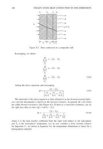
q a T 1 T 2 T 3 T 4
h, T a

x 1 x 2 x 3
Figure 4.2 Heat conduction in a composite wall

Rearranging, we obtain

Q
=−(T 2 − T 1 )
k 1 A
x 1
Q
k 2 A =−(T 3 − T 2 )

x 2
Q
=−(T 4 − T 3 ) (4.8)
k 3 A
x 3
Adding the above equations and rearranging,
(T 1 − T 4 )
(4.9)
Q =
x 1 x 2 x 3
+ +
k 1 A k 2 A k 3 A
The numerator in the above equation is often referred to as the thermal potential differ-
ence and the denominator is known as the thermal resistance. In general, all x/kA terms
are called thermal resistances (See Figure 4.2). If there is a convective resistance, say on
the right face, then we have (Q = hA(T 4 − T a )).

(T 1 − T a )
Q = (4.10)
x 1 x 2 x 3 1
+ + +
k 1 A k 2 A k 3 A hA
where h is the heat transfer coefficient from the right wall surface to the atmosphere
and T a is the atmospheric temperature. Let us now consider a finite element solution
for Equation 4.1. As shown in Equation 4.6, the temperature distribution is linear for a
homogeneous material.