Page 116 - Fundamentals of The Finite Element Method for Heat and Fluid Flow

STEADY STATE HEAT CONDUCTION IN ONE DIMENSION
108
element connecting i and j can be written as
T
[K] = [B] [D][B]d

k 1 −1

= (N i A i + N j A j ) dx
l l 2 −1 1
k A i + A j 1 −1
= (4.25)
l 2 −1 1
where l is the distance between i and j. In the above equation, it has been assumed that
convection is ignored.
Thus, when the area varies linearly, we can substitute an average area value and use the
constant area formulation if there is no heat dissipation from the perimeter. This assumption
will not hold good if the body is circular in cross section, in which case the cross-sectional
area varies quadratically with the axial distance. This case can be dealt with by the use of
a quadratic variation within the element.
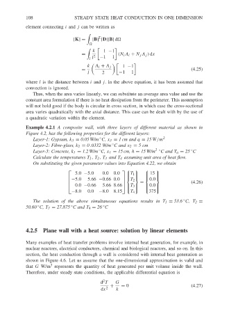
Example 4.2.1 A composite wall, with three layers of different material as shown in
Figure 4.2, has the following properties for the different layers:
◦
Layer-1: Gypsum, k 3 = 0.05 W/m C, x 3 = 1 cm and q = 15 W/m 2
Layer-2: Fibre-glass, k 2 = 0.0332 W/m C and x 2 = 5cm
◦
◦
◦
Layer-3: Concrete, k 1 = 1.2 W/m C, x 1 = 15 cm, h = 15 W/m 2 ◦ C and T a = 25 C
Calculate the temperatures T 1 , T 2 , T 3 and T 4 assuming unit area of heat flow.
On substituting the given parameter values into Equation 4.22, we obtain
     
5.0 −5.0 0.0 0.0
T 1  15 
   
−5.0 5.66 −0.66 0.0    0.0 
  T 2
  = (4.26)

 0.0 −0.66 5.66 8.66 T 3 0.0
   
−8.0 0.0 −8.0 8.15    375 
T 4
◦
The solution of the above simultaneous equations results in T 1 = 53.6 C, T 2 =
50.60 C, T 3 = 27.875 C and T 4 = 26 C
◦
◦
◦
4.2.5 Plane wall with a heat source: solution by linear elements
Many examples of heat transfer problems involve internal heat generation, for example, in
nuclear reactors, electrical conductors, chemical and biological reactors, and so on. In this
section, the heat conduction through a wall is considered with internal heat generation as
shown in Figure 4.6. Let us assume that the one-dimensional approximation is valid and
3
that G W/m represents the quantity of heat generated per unit volume inside the wall.
Therefore, under steady state conditions, the applicable differential equation is
2
d T G
+ = 0 (4.27)
dx 2 k