Page 119 - Fundamentals of The Finite Element Method for Heat and Fluid Flow

STEADY STATE HEAT CONDUCTION IN ONE DIMENSION
Table 4.1 Summary of re-
sults–temperatures
T FEM ( C) Exact ( C) 111
◦
◦
T 1 46.43 46.43
T 2 46.03 46.03
44.83 44.82
T 3
T 4 42.82 42.81
40.0 40.0
T 5
◦
Applying the boundary condition, T 5 = 40 , the modifications are necessary to retain
the symmetry of the stiffness matrix, as discussed in Chapter 3.
    

2800 −2800 0.0 1125
 
0.00.0  T 1
   
−2800 5600 5600    2250 
     
 
0.00.0 T 2
 
 0.0 −2800 5600 −2800 0.0  T 3 = 2250 (4.38)
     
 0.0 0.0 −2800 5600 0.0 T 4   
  
2250 + 2800(40)
   
0.0 0.0 0.0 0.01    40 
T 5
Solving the above system of equations, we obtain the temperature distribution as shown
in Table 4.1.
We observe that the finite element method results are either very close or equal to the
exact solution. The method can be extended for the case of either a known wall heat flux,
or a convection boundary condition at the wall, as shown in Example 4.2.3.
Example 4.2.3 In Example 4.2.2, the left-hand face is insulated and the right-hand face is
◦
subjected to a convection environment at 93 C with a surface heat transfer coefficient of
570 W/m 2 ◦ C. Determine the temperature distribution within the wall.
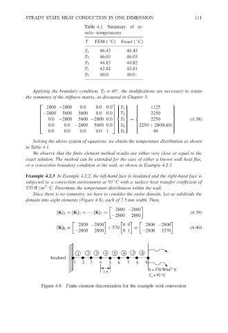
Since there is no symmetry, we have to consider the entire domain. Let us subdivide the
domain into eight elements (Figure 4.8), each of 7.5 mm width. Then,

2800 −2800
[K] 1 = [K] 2 = ··· [K] 7 = (4.39)
−2800 2800

2800 −2800 00 2800 −2800
[K] 8 = + 570 = (4.40)
−2800 2800 01 −2800 3370
1 2 3 4 5 6 7 8
Insulated
1 2 3 4 5 6 7 8 9
2
h = 570 W/m °C
7.5
T = 93 °C
a
Figure 4.8 Finite element discretization for the example with convection