Page 122 - Fundamentals of The Finite Element Method for Heat and Fluid Flow

STEADY STATE HEAT CONDUCTION IN ONE DIMENSION
114
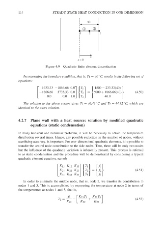
1 30 2
1 2 3

x
x = 0

Figure 4.9 Quadratic finite element discretization

◦
Incorporating the boundary condition, that is, T 3 = 40 C, results in the following set of
equations:
    

1633.33 −1866.66 0.0 T 1
 1500 − 233.33(40) 
−1866.66 3733.33 0.0 = 6000 + 1866.66(40) (4.50)
  T 2
0.0 0.0 1.0    40.0 
T 3
◦
◦
The solution to the above system gives T 1 = 46.43 C and T 2 = 44.82 C, which are
identical to the exact solution.
4.2.7 Plane wall with a heat source: solution by modified quadratic
equations (static condensation)

In many transient and nonlinear problems, it will be necessary to obtain the temperature
distribution several times. Hence, any possible reduction in the number of nodes, without
sacrificing accuracy, is important. For one- dimensional quadratic elements, it is possible to
transfer the central node contribution to the side nodes. Thus, there will be only two nodes
but the influence of the quadratic variation is inherently present. This process is referred
to as static condensation and the procedure will be demonstrated by considering a typical
quadratic element equation, namely,

     
K 11 K 12 K 13 T 1
f 1
 K 21 K 22 K 23  T 2 = f 2 (4.51)
   
K 31 K 32 K 33 T 3 f 3
In order to eliminate the middle node, that is, node 2, we transfer its contribution to
nodes 1 and 3. This is accomplished by expressing the temperature at node 2 in terms of
the temperatures at nodes 1 and 3, that is,

f 2 K 21 T 1 K 23 T 3
T 2 = − + (4.52)
K 22 K 22 K 22