Page 125 - Fundamentals of The Finite Element Method for Heat and Fluid Flow

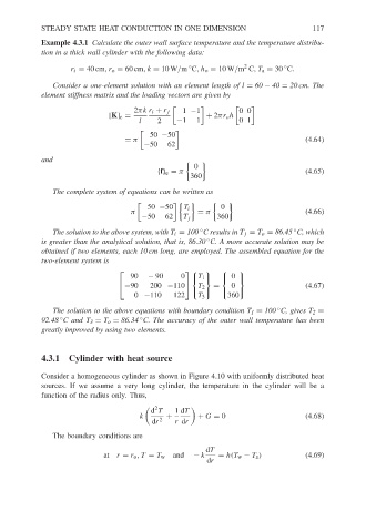
STEADY STATE HEAT CONDUCTION IN ONE DIMENSION
Example 4.3.1 Calculate the outer wall surface temperature and the temperature distribu-
tion in a thick wall cylinder with the following data:
2
◦
◦
r i = 40 cm,r o = 60 cm,k = 10 W/m C,h o = 10 W/m C,T a = 30 C. 117
Consider a one-element solution with an element length of l = 60 − 40 = 20 cm. The
element stiffness matrix and the loading vectors are given by

2πk r i + r j 1 −1 00
[K] e = + 2πr o h
l 2 −1 1 01

50 −50
= π (4.64)
−50 62
and

0
{f} e = π (4.65)
360
The complete system of equations can be written as

50 −50 T i 0
π = π (4.66)
−50 62 T j 360
◦
The solution to the above system, with T i = 100 C results in T j = T o = 86.45 C, which
◦
◦
is greater than the analytical solution, that is, 86.30 C. A more accurate solution may be
obtained if two elements, each 10 cm long, are employed. The assembled equation for the
two-element system is
     
90 − 90
 0 
0 T 1
−90 200 −110 0 (4.67)
  T 2 =
0 −110 122    360 
T 3
◦
The solution to the above equations with boundary condition T 1 = 100 C, gives T 2 =
◦
◦
92.48 C and T 3 = T o = 86.34 C. The accuracy of the outer wall temperature has been
greatly improved by using two elements.
4.3.1 Cylinder with heat source
Consider a homogeneous cylinder as shown in Figure 4.10 with uniformly distributed heat
sources. If we assume a very long cylinder, the temperature in the cylinder will be a
function of the radius only. Thus,

d T 1 dT
2
k + + G = 0 (4.68)
dr 2 r dr
The boundary conditions are
dT
at r = r o ,T = T w and − k = h(T w − T a ) (4.69)
dr