Page 130 - Fundamentals of The Finite Element Method for Heat and Fluid Flow

STEADY STATE HEAT CONDUCTION IN ONE DIMENSION
122
The forcing vector for this problem is

T T T
{f}= G[N] A dx − q[N] dA s + hT a [N] dA s (4.92)
l A s A s
where G is the heat source per unit volume, q is the heat flux, h is the heat transfer
coefficient and T a is the atmospheric temperature. Integrating, we obtain
Gl 2A i + A j ql 2P i + P j hT a l 2P i + P j

0
{f}= − + + hT a A (4.93)
6 A i + 2A j 6 P i + 2P j 6 P i + 2P j 1
The last contribution is valid only for the element at the end face with area A. For all
other elements, this last convective term is zero.
Example 4.4.1 Let us consider an example with the fin tapering linearly from a thickness
of 2 mm at the base to 1 mm at the tip (see Figure 4.14). Also, the tip loses heat to the
ambient with convection, with a heat transfer coefficient, h, = 120 W/m 2 ◦ C and atmospheric
temperature, T a , = 25 C. Determine the temperature distribution if the base temperature
◦
◦
is maintained at 100 C. The total length of the fin, L, is 20 mm and the width, b is 3 mm.
Assume the thermal conductivity of the material is equal to 200 W/m C.
◦
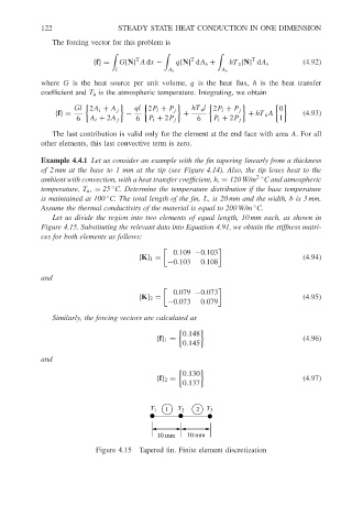
Let us divide the region into two elements of equal length, 10 mm each, as shown in
Figure 4.15. Substituting the relevant data into Equation 4.91, we obtain the stiffness matri-
ces for both elements as follows:

0.109 −0.103
[K] 1 = (4.94)
−0.103 0.108
and

0.079 −0.073
[K] 2 = (4.95)
−0.073 0.079
Similarly, the forcing vectors are calculated as

0.148
{f} 1 = (4.96)
0.145
and
0.130

{f} 2 = (4.97)
0.137

T 1 1 T 2 2 T 3

10 mm 10 mm
Figure 4.15 Tapered fin. Finite element discretization