Page 127 - Fundamentals of The Finite Element Method for Heat and Fluid Flow

STEADY STATE HEAT CONDUCTION IN ONE DIMENSION
2
2
1
1
2
T a = 20 °C
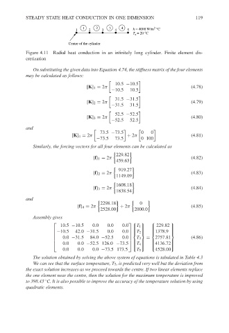
Centre of the cylinder 3 3 4 4 5 h = 4000 W/m °C 119
Figure 4.11 Radial heat conduction in an infinitely long cylinder. Finite element dis-
cretization
On substituting the given data into Equation 4.74, the stiffness matrix of the four elements
may be calculated as follows:

10.5 −10.5
[K] 1 = 2π (4.78)
−10.5 10.5

31.5 −31.5
[K] 2 = 2π (4.79)
−31.5 31.5

52.5 −52.5
[K] 3 = 2π (4.80)
−52.5 52.5
and

73.5 −73.5 0 0
[K] 4 = 2π + 2π (4.81)
−73.5 73.5 0 100
Similarly, the forcing vectors for all four elements can be calculated as

229.82
{f} 1 = 2π (4.82)
459.63

919.27
{f} 2 = 2π (4.83)
1149.09
1608.18

{f} 3 = 2π (4.84)
1838.54
and

2298.18 0
{f} 4 = 2π + 2π (4.85)
2528.00 2000.0
Assembly gives
     
10.5 −10.5 0.0 0.0
 229.82 
0.0 T 1
   
 −10.5 42.0 −31.5 0.0    
 1378.9 

  
0.0   T 2
 
0.0 −31.5 84.0 −52.5 0.0 2757.81 (4.86)
  T 3 =
     
  
 0.0 0.0 −52.5 126.0 −73.5 T 4   
4136.72
   
0.0 0.0 0.0 −73.5 173.5    4528.00 
T 5
The solution obtained by solving the above system of equations is tabulated in Table 4.3
We can see that the surface temperature, T 5 , is predicted very well but the deviation from
the exact solution increases as we proceed towards the centre. If two linear elements replace
the one element near the centre, then the solution for the maximum temperature is improved
◦
to 398.43 C. It is also possible to improve the accuracy of the temperature solution by using
quadratic elements.