Page 120 - Fundamentals of The Finite Element Method for Heat and Fluid Flow

STEADY STATE HEAT CONDUCTION IN ONE DIMENSION
112
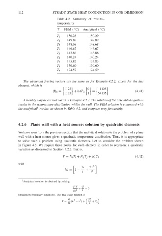
Summary of results–
Table 4.2
temperatures
T FEM ( C) Analytical ( C)
◦
◦
T 1 150.28 150.29
T 2 149.88 149.89
148.68 148.68
T 3
T 4 146.67 146.67
143.86 143.86
T 5
T 6 140.24 140.24
T 7 135.82 135.83
T 8 130.60 130.60
T 9 124.59 124.59
The elemental forcing vectors are the same as for Example 4.2.2, except for the last
element, which is

1125 0 1125
{f} 8 = + hAT a = (4.41)
1125 1 54135
Assembly may be carried out as in Example 4.2.2. The solution of the assembled equation
results in the temperature distribution within the wall. The FEM solution is compared with
1
the analytical results, as shown in Table 4.2, and compare very favourably.

4.2.6 Plane wall with a heat source: solution by quadratic elements

We have seen from the previous section that the analytical solution to the problem of a plane
wall with a heat source gives a quadratic temperature distribution. Thus, it is appropriate
to solve such a problem using quadratic elements. Let us consider the problem shown
in Figure 4.6. We require three nodes for each element in order to represent a quadratic
variation as discussed in Section 3.2.2, that is,

T = N i T i + N j T j + N k T k (4.42)
with
3x 2x
2
N i = 1 − +
l l 2
1 Analytical solution is obtained by solving
2
d T G
+ = 0
dx 2 k
subjected to boundary conditions. The final exact relation is
G 2 2 GL
T = (L − x ) + + T a
2k h