Page 115 - Fundamentals of The Finite Element Method for Heat and Fluid Flow

STEADY STATE HEAT CONDUCTION IN ONE DIMENSION
Assembly gives (see Appendix C)
k 1 A

− k 1 A 0 0  107
 x 1 x 1 
     
 k 1 A k 1 A k 2 A k 1 A 
− + − 0    
  T 1  qA 
     
x 1 x 1 x 2 x 2  T 2 0

= (4.22)
k 2 A k 2 A k 3 A k 3 A
 
  T 3  0 
0    
 − +     
 T 4 hAT a
x 2 x 1 x 3 x 3

 
k 3 A k 3 A
 
0 0 − + hA
x 3 x 3
A solution of the above system of simultaneous equations will result in the values of
T 1 , T 2 , T 3 and T 4 . In a similar way, we can extend this solution method to any number of
materials that might constitute a composite wall. Note that the heat flux imposed on the
left-hand face is q.
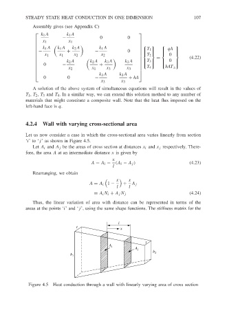
4.2.4 Wall with varying cross-sectional area
Let us now consider a case in which the cross-sectional area varies linearly from section
‘i’to‘j’ as shown in Figure 4.5.
Let A i and A j be the areas of cross section at distances x i and x j respectively. There-
fore, the area A at an intermediate distance x is given by
x
A = A i − (A i − A j ) (4.23)
l
Rearranging, we obtain
x x

A = A i 1 − + A j
l l
= A i N i + A j N j (4.24)
Thus, the linear variation of area with distance can be represented in terms of the
areas at the points ‘i’ and ‘j’, using the same shape functions. The stiffness matrix for the
l
t
x

t
A i
A j
b
b 1 2

Figure 4.5 Heat conduction through a wall with linearly varying area of cross section