Page 113 - Fundamentals of The Finite Element Method for Heat and Fluid Flow

STEADY STATE HEAT CONDUCTION IN ONE DIMENSION
i
T i
l j h, T a 105
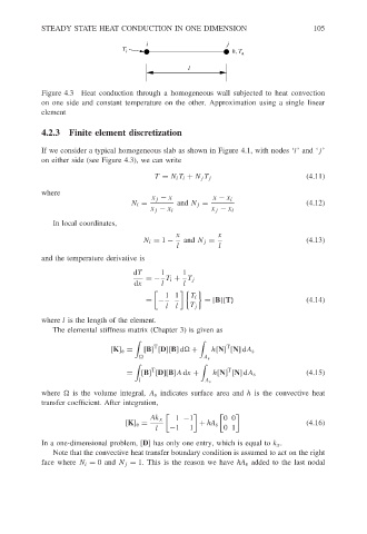
Figure 4.3 Heat conduction through a homogeneous wall subjected to heat convection
on one side and constant temperature on the other. Approximation using a single linear
element

4.2.3 Finite element discretization

If we consider a typical homogeneous slab as shown in Figure 4.1, with nodes ‘i’ and ‘j’
on either side (see Figure 4.3), we can write

T = N i T i + N j T j (4.11)

where
x j − x x − x i
N i = and N j = (4.12)
x j − x i x j − x i
In local coordinates,
x x
N i = 1 − and N j = (4.13)
l l
and the temperature derivative is
dT 1 1
=− T i + T j
dx l l

1 1 T i
= − = [B]{T} (4.14)
l l T j
where l is the length of the element.
The elemental stiffness matrix (Chapter 3) is given as

T T
[K] e = [B] [D][B]d
+ h[N] [N]dA s

A s

T T
= [B] [D][B]A dx + h[N] [N]dA s (4.15)
l A s
where
is the volume integral, A s indicates surface area and h is the convective heat
transfer coefficient. After integration,

Ak x 1 −1 00
[K] e = + hA s (4.16)
l −1 1 01
In a one-dimensional problem, [D] has only one entry, which is equal to k x .
Note that the convective heat transfer boundary condition is assumed to act on the right
face where N i = 0and N j = 1. This is the reason we have hA s added to the last nodal