Page 114 - Fundamentals of The Finite Element Method for Heat and Fluid Flow

STEADY STATE HEAT CONDUCTION IN ONE DIMENSION
106
equation in Equation 4.16. In the plane wall problems considered here, the cross-sectional
area A and convective surface area A s are equal.
The forcing vector can be written as

T T T
{f} e = G[N] d
− q[N] dA s + hT a [N] dA s (4.17)

A s A s
where G is the internal heat generation per unit volume, q is the boundary surface heat flux
and T a is the atmospheric temperature. If G = 0, then there is no heat generation inside
the slab. The no heat flux boundary condition is denoted by q = 0. If neither internal
heat generation nor external heat flux boundary conditions occur, then the finite element
equation for a homogeneous slab (Figure 4.3) with only two nodes becomes
k x A 1 −1 00 T i 0

+ hA = (4.18)
l −1 1 01 T j hT a A
The element equations can now be written for each slab of the composite wall shown
in Figure 4.2 separately and may be assembled. If we assume a discretization as shown in
Figure 4.4, we obtain the following element equations:
Element 1—(Slab 1)
k 1 A k 1 A
 
−
 x 1 x 1  {f} 1 = qA (4.19)
 ;
k 1 A k 1 A 0
[K] 1 = 
−
x 1 x 1
Element 2—(Slab 2)
k 2 A k 2 A
 
−
 x 2 x 2  0
[K] 2 =   ; {f} 2 = (4.20)
k 2 A k 2 A 0
 
−
x 2 x 2
Element 3—(Slab 3)
k 3 A k 3 A
 
−
x 3 x 3
  0
[K] 3 =   ; {f} 3 = (4.21)
 k 3 A k 3 A  hAT a
− + hA
x 3 x 3
1 1 2 2 3 3 4
q h, T a
x 1 x 2 x 3

L
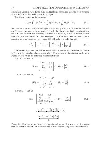
Figure 4.4 Heat conduction through a composite wall subjected to heat convection on one
side and constant heat flux on the other side. Approximation using three linear elements