Page 117 - Fundamentals of The Finite Element Method for Heat and Fluid Flow

STEADY STATE HEAT CONDUCTION IN ONE DIMENSION

T o 109

T w T w

x =−L x = 0 x =+L
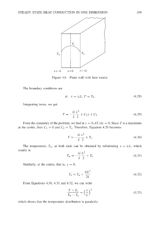
Figure 4.6 Plane wall with heat source

The boundary conditions are

at x =±L, T = T w (4.28)

Integrating twice, we get

G x 2
T =− + C 1 x + C 2 (4.29)
k 2
From the symmetry of the problem, we find at x = 0, dT/dx = 0. Since T is a maximum
at the centre, then C 1 = 0and C 2 = T o . Therefore, Equation 4.29 becomes
G x 2
T =− + T o (4.30)
k 2
The temperature, T w , at both ends can be obtained by substituting x =±L,which
results in
G L 2
T w =− + T o (4.31)
k 2
Similarly, at the centre, that is, x = 0,

GL 2
T o = T w + (4.32)
2k
From Equations 4.30, 4.31 and 4.32, we can write

x
2
T − T o
= (4.33)
T w − T o L
which shows that the temperature distribution is parabolic.