Page 198 - Fundamentals of The Finite Element Method for Heat and Fluid Flow

190
we can write using a Taylor series expansion as follows:
2
2
n
∂ φ x
n n ∂φ x 1 CONVECTION HEAT TRANSFER
1
φ | x 1 − x 1 = φ | x 1 − + 2 − ··· (7.78)
∂x 1 1! ∂x 2!
1
Similarly, the diffusion term is expanded as
n
∂ ∂φ n ∂ ∂φ n ∂ ∂ ∂φ
k | x 1 − x 1 = k | x 1 − k x (7.79)
∂x ∂x ∂x 1 ∂x 1 ∂x 1 ∂x 1 ∂x 1
1 1
On substituting Equations 7.78 and 7.79 into Equation 7.77, we obtain (higher-order
terms being neglected) the following expression:
2
2
φ n+1 − φ n x ∂φ n x ∂ φ n ∂ ∂φ n
=− + + k (7.80)
t t ∂x 1 2 t ∂x 2 ∂x 1 ∂x 1
1
In this case, all the terms are evaluated at the position x 1 , and not at two positions as
in Equation 7.77. If the flow velocity is u 1 , we can write x = u 1 t. Substituting into
Equation 7.80, we obtain the semi-discrete form as
2
φ n+1 − φ n ∂φ n 2 t ∂ φ n ∂ ∂φ n
=−u 1 + u 1 + k (7.81)
t ∂x 1 2 ∂x 2 ∂x 1 ∂x 1
1
By carrying out a Taylor series expansion (see Figure 7.8), the convection term reap-
pears in the equation along with an additional second-order term. This second-order term
acts as a smoothing operator that reduces the oscillations arising from the spatial discretiza-
tion of the convection terms. The equation is now ready for spatial approximation.
The following linear spatial approximation of the scalar variable φ in space is used to
approximate Equation 7.81:
φ = N i φ i + N j φ j = [N]{φ} (7.82)
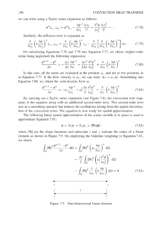
where [N] are the shape functions and subscripts i and j indicate the nodes of a linear
element as shown in Figure 7.9. On employing the Galerkin weighting to Equation 7.81,
we obtain
φ n+1 − φ n ∂φ n
[N] T d
+ [N] T u 1 d

t
∂x 1
n
!
2
t T 2 ∂ φ
− [N] u 1 d
2
∂x 1 2
∂ ∂φ
− [N] T k d
= 0 (7.83)

∂x 1 ∂x 1

i j
l

Figure 7.9 One-dimensional linear element