Page 203 - Fundamentals of The Finite Element Method for Heat and Fluid Flow

CONVECTION HEAT TRANSFER
u = constant
1
f = 0
Inlet
Exit
L f = 1 195
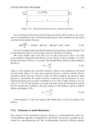
Figure 7.10 One-dimensional convection–diffusion problems

For a one-dimensional domain with more than one element, all the matrices and vectors
need to be assembled in order to obtain the global matrices. Once assembled, the discretized
one-dimensional equation becomes

{φ} n n n n n
[M] =−[C]{φ} − [K 1 ]{φ} − [K 2 ]{φ} +{f 1 } +{f 2 } (7.102)
t
Letusnowconsiderasimpleone-dimensionalconvectionproblem,asgiveninFigure 7.10,
to demonstrate the effect of a discretization with and without the CG scheme.
The scalar variable value at the inlet is φ = 0, and at the exit its value is 1.0. This
scalar variable is transported in the direction of the velocity as shown in Figure 7.10. Note
that the convection velocity u 1 is constant. The element Peclet number for this problem is
defined as
u 1 h
Pe = (7.103)
2k
where h is the element size in the flow direction, which, in one dimension is the local
element length. Figure 7.11 shows the comparison between a solution with the CG dis-
cretization scheme and one without it. Only two Peclet numbers are shown in these
diagrams to demonstrate the spatial oscillations without the CG discretization. As seen,
both discretizations give no spatial oscillations at a Pe value of unity. However, at a Pe
value of 1.5, the CG discretization is accurate and stable, while the discretization without
the CG term becomes oscillatory. The exact solution to this problem is given as follows
(Brooks and Hughes 1982):
u 1 x 1
1 − e k
φ = (7.104)
u 1 L
1 − e k
In this equation, L is the total length of the domain and x 1 is the local length of the
domain.

7.4.2 Extension to multi-dimensions

The extension of the characteristic Galerkin scheme to a multi-dimensional scalar con-
vection-diffusion equation is straightforward and follows the previous procedure as dis-
cussed for a one-dimensional case. The two-dimensional convection–diffusion equation