Page 232 - Fundamentals of The Finite Element Method for Heat and Fluid Flow

CONVECTION HEAT TRANSFER
224
within a fluid, but will not be considered within this text. Buoyancy-driven convection is
present in most flow situations; however, its significance can vary according to the situation.
For instance, in a situation in which a hot surface and a cold fluid interact, without any
other external force, a buoyancy-driven convection pattern will develop. Examples include
radiators inside a cold room, most solar appliances, some cooling applications of electronic
devices and finally phase change applications (Lewis et al. 1995a; Ravindran and Lewis
1998; Usmani et al. 1992b,a).
The principles of buoyancy-driven convection are simple. A local temperature difference
creates a local density difference within the fluid and results in fluid motion because of the
local density variation. Although the principles are simple, the development of an accurate
numerical solution for such buoyancy-driven flows is far from simple. This is mainly due
to the very slow flow rates involved, which are often marked with turbulence, which again
complicates the numerical prediction.
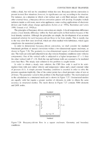
In order to demonstrate buoyancy-driven convection, we shall consider the standard
benchmark problem of natural convection within a two-dimensional square enclosure, as
shown in Figure 7.26. The geometry is a two-dimensional square of non-dimensional unit
size. The walls are solid and subjected to no-slip velocity boundary conditions (zero-velocity
components). One of the vertical walls is subjected to a higher temperature (T =1)than
the other vertical wall (T = 0). Both the top and bottom walls are assumed to be insulated
(zero heat flux). The steady state solution to this problem is sought herein.
In order to obtain a steady state solution, the CBS flow code is used in its semi-
implicit form with zero initial velocity and temperature values and a small constant value
of pressure (0.1). A simple pressure boundary condition is essential in order to solve the
pressure equations implicitly. One of the corner points has a fixed pressure value of zero at
all times. The parameter varied in this problem is the Rayleigh number. The mesh employed
in the calculations is a structured mesh and is shown in Figure 7.27. Unstructured meshes
are equally valid but require a greater number of elements in order to obtain the same
accuracy as structured meshes. The mesh shown in Figure 7.27 contains 5000 elements
and 2601 nodes.

Insulated

u = u = 0
1
2
= 0 = 0
= u 2 = u 2
T = 1 T = 0
u 1 u 1

u = u = 0
2
1
Insulated
Figure 7.26 Buoyancy-driven flow in a square enclosure. Geometry and boundary
conditions