Page 277 - Fundamentals of The Finite Element Method for Heat and Fluid Flow

SOME EXAMPLES OF FLUID FLOW AND HEAT TRANSFER PROBLEMS

(a) Mesh5 (b) Mesh6 269
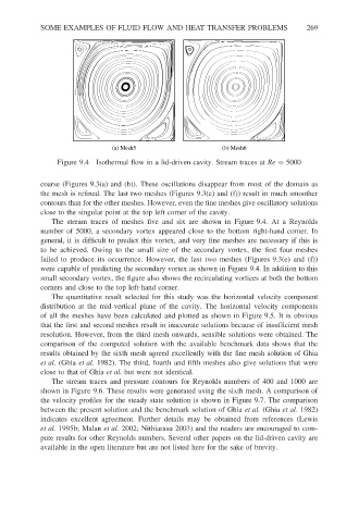
Figure 9.4 Isothermal flow in a lid-driven cavity. Stream traces at Re = 5000

coarse (Figures 9.3(a) and (b)). These oscillations disappear from most of the domain as
the mesh is refined. The last two meshes (Figures 9.3(e) and (f)) result in much smoother
contours than for the other meshes. However, even the fine meshes give oscillatory solutions
close to the singular point at the top left corner of the cavity.
The stream traces of meshes five and six are shown in Figure 9.4. At a Reynolds
number of 5000, a secondary vortex appeared close to the bottom right-hand corner. In
general, it is difficult to predict this vortex, and very fine meshes are necessary if this is
to be achieved. Owing to the small size of the secondary vortex, the first four meshes
failed to produce its occurrence. However, the last two meshes (Figures 9.3(e) and (f))
were capable of predicting the secondary vortex as shown in Figure 9.4. In addition to this
small secondary vortex, the figure also shows the recirculating vortices at both the bottom
corners and close to the top left-hand corner.
The quantitative result selected for this study was the horizontal velocity component
distribution at the mid-vertical plane of the cavity. The horizontal velocity components
of all the meshes have been calculated and plotted as shown in Figure 9.5. It is obvious
that the first and second meshes result in inaccurate solutions because of insufficient mesh
resolution. However, from the third mesh onwards, sensible solutions were obtained. The
comparison of the computed solution with the available benchmark data shows that the
results obtained by the sixth mesh agreed excellently with the fine mesh solution of Ghia
et al. (Ghia et al. 1982). The third, fourth and fifth meshes also give solutions that were
close to that of Ghia et al. but were not identical.
The stream traces and pressure contours for Reynolds numbers of 400 and 1000 are
shown in Figure 9.6. These results were generated using the sixth mesh. A comparison of
the velocity profiles for the steady state solution is shown in Figure 9.7. The comparison
between the present solution and the benchmark solution of Ghia et al. (Ghia et al. 1982)
indicates excellent agreement. Further details may be obtained from references (Lewis
et al. 1995b; Malan et al. 2002; Nithiarasu 2003) and the readers are encouraged to com-
pute results for other Reynolds numbers. Several other papers on the lid-driven cavity are
available in the open literature but are not listed here for the sake of brevity.