Page 281 - Fundamentals of The Finite Element Method for Heat and Fluid Flow

273
SOME EXAMPLES OF FLUID FLOW AND HEAT TRANSFER PROBLEMS
The second mesh was generated by adapting the mesh for the solution generated on a
coarse mesh (see reference (Nithiarasu and Zienkiewicz 2000) for details) as shown in
Figure 9.9(b). It should be observed that the adapted mesh is not fine in the region close
to the recirculation zone, and this may lead to inaccuracies in that region. However, the
use of unstructured meshes was preferred so that the flexibility of the method could easily
be proven.
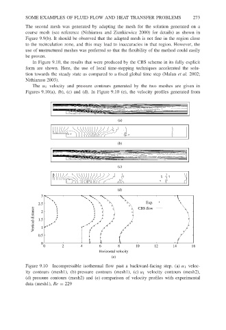
In Figure 9.10, the results that were produced by the CBS scheme in its fully explicit
form are shown. Here, the use of local time-stepping techniques accelerated the solu-
tion towards the steady state as compared to a fixed global time step (Malan et al. 2002;
Nithiarasu 2003).
The u 1 velocity and pressure contours generated by the two meshes are given in
Figures 9.10(a), (b), (c) and (d). In Figure 9.10 (e), the velocity profiles generated from

(a)

(b)

(c)

(d)
3
Exp.
2.5 CBS flow
Vertical distance 1.5 2

0.5 1
0
0 2 4 6 8 10 12 14 16
Horizontal velocity
(e)
Figure 9.10 Incompressible isothermal flow past a backward-facing step. (a) u 1 veloc-
ity contours (mesh1), (b) pressure contours (mesh1), (c) u 1 velocity contours (mesh2),
(d) pressure contours (mesh2) and (e) comparison of velocity profiles with experimental
data (mesh1), Re = 229