Page 284 - Fundamentals of The Finite Element Method for Heat and Fluid Flow

SOME EXAMPLES OF FLUID FLOW AND HEAT TRANSFER PROBLEMS
276

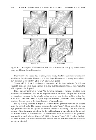
(a) Re = 50 (b) = 100

(c) Re = 400 (d) Re = 1000
Figure 9.13 Incompressible isothermal flow in a double-driven cavity. u 2 velocity con-
tours for different Reynolds numbers

Theoretically, the steady state solution, if one exists, should be symmetric with respect
to either of the diagonals. However, at higher Reynolds numbers, a steady state solution
may not exist as reported by Zhou et al. (Zhou et al. 2003).
Figures 9.12, 9.13 and 9.14 show the contours of all the three variables for different
Reynolds numbers. From these contours it is clear that the solution obtained was symmetric
with respect to the diagonals.
The u 1 velocity contours in Figure 9.12 show the existence of strong u 1 gradients close
to the top and the bottom lids. As the Reynolds number increases, this gradient increases
in strength as indicated by the closely packed contours near the top and the bottom lids
at Re = 400 and 1000. Also, at higher Reynolds numbers (Re = 400, 1000), stronger u 1
gradients develop close to the inward corners of the enclosure.
The u 2 velocity contours in Figure 9.13 show steeper gradients close to the corners
along the vertical walls. The pressure contours shown in Figure 9.14 are marked with very
high gradients close to the top and the bottom corners of the cavity. This was expected
because of the singularity introduced by the sudden change in the velocity at the top and
the bottom corners. A comparison of the unstructured mesh solution with the published
structured fine mesh solution (Zhou et al. 2003) is shown in Figure 9.15. It is clear that both
the finite element solution on unstructured meshes and the fine structured mesh solution
are almost identical.