Page 288 - Fundamentals of The Finite Element Method for Heat and Fluid Flow

SOME EXAMPLES OF FLUID FLOW AND HEAT TRANSFER PROBLEMS
280
0.6
0.4 CBS flow
Sampaio et al.
0.2
u 3 at exit 0
−0.2
−0.4
−0.6
0 10 20 30 40 50 60 70
Time

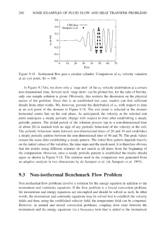
Figure 9.18 Isothermal flow past a circular cylinder. Comparison of u 3 velocity variation
at an exit point, Re = 100

In Figure 9.17(b), we show only a ‘snap shot’ of the u 1 velocity distribution at a certain
non-dimensional time. Several such ‘snap shots’ can be plotted but, for the sake of brevity,
only one sample solution is given. Obviously, this restricts the discussion on the physical
nature of the problem. Since this is an established test case, readers can find sufficient
details from other works. We, however, provide the distribution of u 3 with respect to time
at an exit point of the domain in Figure 9.18. The exit point is selected at the domain
horizontal centre line on the exit plane. As anticipated, the velocity at the selected exit
point undergoes a steady periodic change with respect to time after establishing a steady
periodic pattern. The initial period of the solution process (up to a non-dimensional time
of about 20) is marked with no sign of any periodic behaviour of the velocity at the exit.
The periodic behaviour starts between non-dimensional times of 20 and 30 and establishes
a steady periodic pattern between the non-dimensional time of 40 and 50. The peak values
remain the same after establishing a steady pattern. The initial flow pattern depends heavily
on the initial values of the variables, the time steps and the mesh used. It is therefore obvious
that the results using different schemes do not match at all times from the beginning of
the computation. However, once a steady periodic pattern is established the results should
agree as shown in Figure 9.18. The solution used in the comparison was generated from
an adaptive analysis in two dimensions by de Sampaio et al. (de Sampaio et al. 1993).

9.3 Non-isothermal Benchmark Flow Problem

Non-isothermal flow problems involve a solution for the energy equation in addition to the
momentum and continuity equations. If the flow problem is a forced convection problem,
the momentum and energy equations are uncoupled and should be solved as such. In other
words, the momentum and continuity equations may be solved first to establish the velocity
fields and then, using the established velocity field, the temperature field can be computed.
However, in natural and mixed convection problems, coupling does exist between the
momentum and the energy equations via a buoyancy term that is added to the momentum