Page 136 - Fundamentals of Water Treatment Unit Processes : Physical, Chemical, and Biological

Screening 91

HLR is by definition: which is essentially the same as the mass removal rate, since
C 0, is obtained by multiplying both sides of Equation
Q Ex5.3.20 by C r . The resulting equation is merely a derivative
(Ex5:3:18)
LQ M r of Equation Ex5.3.20 and is not shown.
HLR ¼
The ‘‘passive’’ variables in Equation Ex5.3.20 may be
Combining (Ex5.3.17) and (Ex5.3.18) gives
consolidated into a single coefficient, K, which must be deter-
mined by pilot plant testing, or from data obtained from a full-
0:5
2rvk(mat)h L (mat) scale plant. The variable, Q M , is also consolidated in the
(Ex5:3:19)
HLR ¼
Q M C r coefficient. The result is an equation that has more utility, i.e.,
Again, to simplify, substitute Equation Ex5.3.13 for h L (mat) 0:5 0:5
to give HLR ¼ Kv h L (Ex5:3:21)
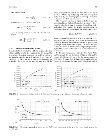
0:5 Figure 5.12a and b shows plots of HLR vs. h L and HLR vs. v,
2rvk(mat)h L
(Ex5:3:20) 4
HLR ¼ respectively for K ¼ 3.6 10 m=s. Figure 5.12a shows that
Q M C r
increasing headloss toward the higher end of practice can
yield significantly higher HLR. Figure 5.12b shows that pro-
viding for a several-fold increase in v can permit significantly
5.5.7.1 Interpretation of Model Results higher HLR, which would therefore be an important variable
Equation Ex5.3.20 says that the HLR for design is a function in operation.
of the variables listed in the equation to the 1=2 power. The By the same token, since A ¼ Q=v, the plots, Figure 5.13a
two design-independent variables are h L and Q M , while v is and b, respectively, are derivatives of Figure 5.12a and b,
an operating variable, and r, k(mat) and C r are ‘‘passive’’ respectively. Figure 5.13a shows that the required area for a
3
variables, i.e., those that are ambient or are otherwise not 0.31 m =s (7 mgd) flow declines exponentially with an
controlled. The mass loading rate per unit area (MLR), increase in headloss applied to the design. Also, if v is applied

0.010 0.010
0.009 0.009
0.008 0.008
0.007
HLR (m 3 /s/m 2 ) 0.006 y=0.006147*x^(0.49875) HLR (m 3 /s/m 2 ) 0.006 y =0.010393*x^(0.48944)
0.007
0.005
0.005
0.004
0.004
0.003
0.002
0.002 Range of 0.003 Range of practice
practice
0.001 0.001
0.000 0.000
0.0 0.5 1.0 1.5 2.0 2.5 3.0 0 0.1 0.2 0.3 0.4 0.5 0.6 0.7 0.8 0.9 1
(a) h (m) (b) ω (rad/s)
L
FIGURE 5.12 Microscreen calculated HLRs for K (50%). (a) HLR versus h L for h L ¼ 0.3 m. (b) HLR versus v for v ¼ 0.1 rad=s.

150 150
y=50.087*x^(–0.49912) y=29.608*x^(–0.48992)

A(net) (m 2 ) 100 A(net) (m 2 ) 100

50
Range of 50
practice Range of practice

0 0
0.0 0.5 1.0 1.5 2.0 2.5 3.0 0.0 0.1 0.2 0.3 0.4 0.5 0.6 0.7 0.8 0.9 1.0
(a) h (m) (b) ω (rad/s)
L
FIGURE 5.13 Microscreen calculated net screen area for K (50%). (a) A(net) versus h L for h L ¼ 0.3 m. (b) A(net) versus v for
v ¼ 0.1 rad=s.