Page 142 - Fundamentals of Water Treatment Unit Processes : Physical, Chemical, and Biological

Sedimentation 97

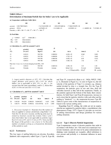
TABLE CDEx6.1
Determination of Maximum Particle Size for Stokes’ Law to be Applicable
(a) Temperature coefficients (Table QR.4)
M0 M1 M2 M3 M4 M5
m(water) 0.0017802356694 5.6132434302E 05 1.0031470384E-06 7.5406393887E 09
r(water) 999.84 6.82560E 02 9.14380E 03 1.02950E 04 1.18880E 06 7.15150E 09
2
3
Formula: y ¼ M0 þ M1 T þ M2 T þ M3 T þ M4 T 4
(b) Fixed data
g ¼ 9.80665 m=s 2 (Table QR.1)
SG s ¼ 2.65 dimensionless
SG f ¼ 1.00 dimensionless

(c) Calculation of v s and R for assumed T and d
D v s
T m(water) r(water)
2
3
(8C) (N s=m ) (kg=m ) (m) (m=s) (mm=s) R
10 0.00131 999.700 0.000010 6.85E 05 0.069 0.001
10 0.00131 999.700 0.000050 1.71E 03 1.71 0.065
10 0.00131 999.700 0.000100 6.85E 03 6.85 0.522
10 0.00131 999.700 0.000150 1.54E 02 15.4 1.76
Final trial in next row involved changing d until R ¼ 1.00
10 0.00131 999.700 0.000124 1.05E 02 10.5 1.00
Assume Formula Formula Assume Stokes’ law Convert Calculate
v s ¼ (1=18)(rg=m)(SG s SG f )d 2 R ¼ rv s d=m

3. Largest particle diameter at 208C, 08C: Calculate the and Type IV, respectively (Katz et al., 1962a; WPCF, 1985,
largest diameter sand particle (SG ¼ 2.65) for which p. 3), illustrated in Figure 6.2. As seen in Figure 6.2, the fall
Stokes’ law is applicable at 208C, 08C, i.e., R 1. An velocity of the particles of Type I is constant, e.g., distance
excerpt from the same spreadsheet, used in 2, shows that settled divided by time is a straight line. For the Type II
d(20) ¼ 0.104 mm and d(0) ¼ 0.152 mm.
suspension, the particles grow in size and, thus, their fall
velocities increase as they fall in the suspension. Finally, as
(c) Calculation of v s and R for assumed T and d
the particles approach the bottom of the basin, their concen-
trations, for both Type I and Type II suspensions, increase to
v s
T m(water) r(water) d such extent that the particles interfere with each other and the
3
2
(8C) (N s=m ) (kg=m ) (m) (m=s) (mm=s) R
settling is ‘‘hindered,’’ i.e., the suspension becomes Type III.
20 0.00100 998.204 0.000104 0.00965457 9.655 1.000 Table 6.2 gives some of the characteristics of suspensions as
0 0.00178 999.840 0.000152 0.011695382 11.70 1.000 found in the various settling units.
Regarding Type IV settling, the solids are not in suspen-
sion but are supported by particles below; consolidation is the
4. Discussion: Example 6.1 illustrates how the numerical phenomenon (Camp, 1937). Figure 6.2 provides an overview
data are applied to various calculations using Stokes’ law. of settling characteristics and design guidelines for various
Note that the dynamic viscosity and the kg units must be settling situations.
related by Newton’s second law relation. Parts 2 and 3
show that Stokes’ law is not applicable to particles larger
than 0.15 mm at 08C and 0.10 mm at 208C. Note also that
the shape of the particle is not a factor in the Reynolds 6.2.3.1 Type I: Discrete Particle Suspensions
number calculation as long as a characteristic dimension
of the particle is used. Type I suspensions consist of discrete particles that settle in
accordance with Stokes’ law. Grit removal in municipal was-
tewater treatment, and silt removal by plain sedimentation in
6.2.3 SUSPENSIONS
drinking water treatment are examples, albeit turbulence is
The four types of settling behaviors are discrete, flocculent, ever present and probably is a dominant influence in most
hindered, and compression, called Type I, Type II, Type III, situations.