Page 298 - Fundamentals of Water Treatment Unit Processes : Physical, Chemical, and Biological

Mixing 253

10 4
BOX 10.3 NAVIER AND STOKES
10 3 A certain amount of mystique is associated with the
Navier–Stokes equation. A brief account of its develop-
10 2 d =10 μm ment (from Rouse and Ince, 1957, pp. 91, 92, 104,
d =1 μm 193–198) may help to gain some familiarity. The equa-
10 1 tion was developed almost in its present form by Louis
J ok /J pk J ok pk Marie Henri Navier (1785–1836). A graduate of Ponts
/J =1
10 0 et Chaussées, he taught there and at Ecole Polytechni-
d=0.1 μm que. In an 1822 paper to the Académie des Sciences,he
10 –1 built on an earlier work by Leonhard Euler (1707–
1783), i.e., that body forces plus pressure gradient
10 –2 equals local acceleration plus advective acceleration.
Navier, however, added a hypothetical molecular attrac-
10 –3 tion, embodied in a term, e. Then, in 1845, Sir George
10 –3 10 –2 10 –1 10 0 10 1 10 2 10 3 10 4 Gabriel Stokes (1819–1903), in a paper before the
–1
G (s ) Royal Society, replaced the coefficient, e, with the
dynamic viscosity, m, giving the equation its current
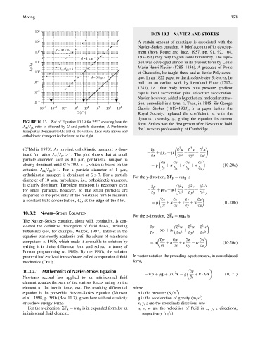
FIGURE 10.13 Plot of Equation 10.19 for 258C showing how the
form. Stokes was the first person after Newton to hold
J ok =J pk ratio is affected by G and particle diameter, d. Perikinetic
the Lucasian professorship at Cambridge.
transport is dominant to the left of the vertical lines with arrows and
orthokinetic transport is dominant to the right.

2 2 2
(O’Melia, 1970). As implied, orthokinetic transport is dom- qp q u q u q u
inant for ratios J ok =J pk > 1. The plot shows that at small qx þ rg x þ m qx 2 þ qy 2 þ qz 2
particle diameter, such as 0.1 mm, perikinetic transport is
1
clearly dominant until G 7000 s , which is basedonthe ¼ r qu þ u qu þ v qu þ w qu (10:20a)
criterion J ok =J pk > 1. For a particle diameter of 1 mm, qt qx qy qz
orthokinetic transport is dominant at G > 7. For a particle
~
For the y-direction, SF y ¼ ma y is
diameter of 10 mm, turbulence, i.e., orthokinetic transport,
is clearly dominant. Turbulent transport is necessary even 2 2 2
qp q v q v q v
for small particles, however, so that small particles are þ rg y þ m þ þ
qy qx 2 qy 2 qz 2
dispersed to the proximity of the resistance film to maintain

a constant bulk concentration, C o , at the edge of the film. qv qv qv qv
¼ r þ u þ v þ w (10:20b)
qt qx qy qz
10.3.2 NAVIER–STOKES EQUATION ~
For the z-direction, SF z ¼ ma z is
The Navier–Stokes equation, along with continuity, is con-
2
2
2
sidered the definitive description of fluid flows, including qp q w q w q w
turbulence (see, for example, Wilcox, 1997). Interest in the qz þ rg z þ m qx 2 þ qy 2 þ qz 2
equation was mostly academic until the advent of mainframe
qw qw qw qw
computers, c. 1958, which made it amenable to solution by ¼ r þ u þ v þ w (10:20c)
writing it in finite difference form and solved in terms of qt qx qy qz
Fortran programming (c. 1960). By the 1990s, the solution
protocol had evolved into software called computational fluid In vector notation the preceding equations are, in consolidated
mechanics (CFD). form,

10.3.2.1 Mathematics of Navier–Stokes Equation 2 qv
rp þ rg þ mr v ¼ r þ v rv (10:21)
Newton’s second law applied to an infinitesimal fluid qt
element equates the sum of the various forces acting on the
element to the inertia force, ma. The resulting differential where
2
equation is the proverbial Navier–Stokes equation (Munson p is the pressure (N=m )
2
et al., 1998, p. 360) (Box 10.3), given here without elasticity g is the acceleration of gravity (m=s )
or surface energy terms. x, y, z are the coordinate directions (m)
~
For the x-direction, SF x ¼ ma x is in expanded form for an u, v, w are the velocities of fluid in x, y, z directions,
infinitesimal fluid element, respectively (m=s)