Page 303 - Fundamentals of Water Treatment Unit Processes : Physical, Chemical, and Biological

258 Fundamentals of Water Treatment Unit Processes: Physical, Chemical, and Biological

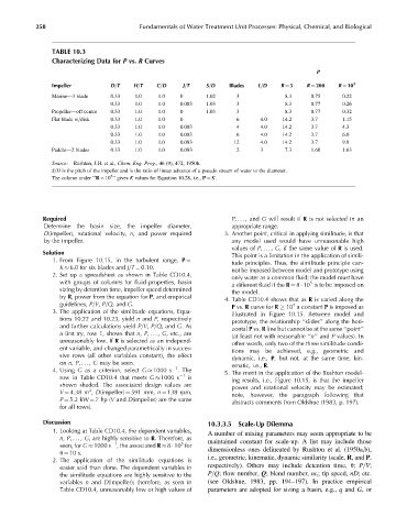
TABLE 10.3
Characterizing Data for P vs. R Curves
P

Impeller D=T H=T C=D J=T S=D Blades L=D R ¼ 5 R ¼ 200 R ¼ 10 5
Marine—3 blade 0.33 1.0 1.0 0 1.02 3 8.3 0.75 0.22
0.33 1.0 1.0 0.083 1.03 3 8.3 0.77 0.26
Propeller—off center 0.33 1.0 1.0 0 1.03 3 8.3 0.77 0.32
Flat blade w=disk 0.33 1.0 1.0 0 6 4.0 14.2 3.7 1.15
0.33 1.0 1.0 0.083 4 4.0 14.2 3.7 4.3
0.33 1.0 1.0 0.083 6 4.0 14.2 3.7 6.0
0.33 1.0 1.0 0.083 12 4.0 14.2 3.7 9.9
Paddle—2 blades 0.33 1.0 1.0 0.083 2 3 7.3 1.60 1.63
Source: Rushton, J.H. et al., Chem. Eng. Prog., 46 (9), 472, 1950b.
S=D is the pitch of the impeller and is the ratio of linear advance of a pseudo stream of water to the diameter.
5
The column under ‘‘R ¼ 10 ’’ gives K values for Equation 10.28, i.e., P ¼ K.

Required P,... , and G will result if R is not selected in an
Determine the basin size, the impeller diameter, appropriate range.
D(impeller), rotational velocity, n, and power required 3. Another point, critical in applying similitude, is that
by the impeller. any model used would have unreasonable high
values of P,.. ., G, if the same value of R is used.
Solution
This point is a limitation in the application of simili-
tude principles. Thus, the similitude principle can-
1. From Figure 10.15, in the turbulent range, P ¼
K 6.0 for six blades and J=T ¼ 0.10.
not be imposed between model and prototype using
2. Set up a spreadsheet as shown in Table CD10.4,
only water as a common fluid; the model must have
with groups of columns for fluid properties, basin 5
a different fluid if the R ¼ 8 10 is to be imposed on
sizing by detention time, impeller speed determined the model.
by R, power from the equation for P, and empirical 4. Table CD10.4 shows that as R is varied along the
guidelines, P=V, P=Q, and G. P vs. R curve for R 10 a constant P is imposed as
4
3. The application of the similitude equations, Equa- illustrated in Figure 10.15. Between model and
tions 10.22 and 10.23, yield n and P, respectively prototype, the relationship ‘‘slides’’ along the hori-
and further calculations yield P=V, P=Q, and G.As zontal P vs. R line but cannot be at the same ‘‘point’’
a first try, row 1, shows that n, P,... , G, etc., are (at least not with reasonable ‘‘n’’ and P values). In
unreasonably low. If R is selected as an independ- other words, only two of the three similitude condi-
ent variable, and changed parametrically in succes- tions may be achieved, e.g., geometric and
sive rows (all other variables constant), the effect dynamic, i.e., P, but not, at the same time, kin-
on n, P,..., G may be seen. ematic, i.e., R.
1
4. Using G as a criterion, select G 1000 s . The 5. The merit in the application of the Rushton model-
row in Table CD10.4 that meets G 1000 s 1 is ing results, i.e., Figure 10.15, is that the impeller
shown shaded. The associated design values are power and rotational velocity may be estimated;
3
V ¼ 4.38 m , D(impeller) ¼ 591 mm, n ¼ 138 rpm, note, however, the paragraph following that
P ¼ 5.2 kW ¼ 7hp(V and D(impeller) are the same abstracts comments from Oldshue (1983, p. 197).
for all rows).
Discussion 10.3.3.5 Scale-Up Dilemma
1. Looking at Table CD10.4, the dependent variables,
A number of mixing parameters may seem appropriate to be
n, P,..., G, are highly sensitive to R. Therefore, as maintained constant for scale-up. A list may include those
1
5
seen, for G 1000 s , the associated R 8 10 for
dimensionless ones delineated by Rushton et al. (1950a,b),
u ¼ 10 s.
i.e., geometric, kinematic, dynamic similarity (scale, R,and P,
2. The application of the similitude equations is
respectively). Others may include detention time, u; P=V;
easier said than done. The dependent variables in
the similitude equations are highly sensitive to the P=Q; flow number, Q; blend number, nt r ; tip speed, nD; etc.
variables n and D(impeller); therefore, as seen in (see Oldshue, 1983, pp. 194–197). In practice empirical
Table CD10.4, unreasonably low or high values of parameters are adopted for sizing a basin, e.g., q and G,or