Page 302 - Fundamentals of Water Treatment Unit Processes : Physical, Chemical, and Biological

Mixing 257

100
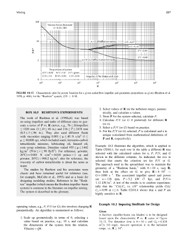
Viscous forces dominate
n=0, R≤300

1
10 1 n=0 (4 baffles/no vortex) J/T=0.17
J/T=0.10
P/F n J/T=0.04

J/T =0.00
1 n≠0 (no baffles/vortex formed)

Proportions of system
D/T=0.33 H/T =1.0 J/T=given
C/D=1.0 W/D =0.33 L/D=0.25 Impeller: 6 flat blades with disk
0
10 0 10 1 10 2 10 3 10 4 10 5 10 6
R

FIGURE 10.15 Characteristic plot for power function for a given radial-flow impeller and geometric proportions as given (Rushton et al.
1950, p. 468); for the ‘‘Rushton’’ system, J=D ¼ 0.10.

2. Select values of R (in the turbulent range), parame-
BOX 10.5 RUSHTON’S EXPERIMENTS trically, and calculate n values.
3. From P for the system selected, calculate P.
The work of Rushton et al. (1950a,b) was based
4. Calculate P=V (or G if preferred) for different R
on using impellers and tanks of different sizes to gen-
(or n).
erate a series of P vs. R curves, e.g., 76 D(impeller)
5. Select a P=V (or G) based on practice.
1220 mm (3 D 48 in.) and 216 T 2438 mm
6. For the P=V (or G) selected, P is calculated and n is
(8.5 T 96 in.). They also used different fluids
2 unique (calculated from mathematical definitions of
with viscosities ranging 0.001 m 40 N s=m (1
P and R, respectively).
m 40,000 cp), which included water, kerosene–carbon
tetrachloride mixtures, lubricating oil, linseed oil,
Example 10.2 illustrates the algorithm, which is applied in
corn syrup solutions. Densities varied 955 r 1442 Table CD10.4; for each row in the table a different R was
3
3
kg=m (59.6 r 90 lb=ft ). For reference, m(water, selected with the calculated values for n, P, P=V, and G
2
208C) 0.001 N s=m ¼ 0.010 poises ¼ 1 cp and shown in the different columns. As indicated, the row is
3
r(water, 208C) ¼ 998.2 kg=m ; also for reference, the
selected that meets the criterion set for P=V or G.
viscosity of carbon tetrachloride is about the same as
The approach used in the spreadsheet was to maintain the
water.
geometry of a ‘‘Rushton basin,’’ with u ¼ 10 s, vary R,
The studies by Rushton and his associates were 5
then look at the effect on G, to give R ¼ 8 10
classic and have remained useful for reference (see, 1 !
G 1000 s . The associated impeller speed and power
for example, McCabe et al., 1993) and as a basis for
designing modeling studies. Reference to the ‘‘Rush- are n ¼ 138 rpm, P ¼ 5.2 kW (7 hp), and P=V
3
1.12 kW=m . A test of the results is to confirm experimen-
ton’’ impeller (which means the Rushton impeller–basin
tally that the ‘‘C(t)=C o vs. t=u’’ relationship yields C(t)=
system) is common in the literature on impeller mixing.
C o 0.99 at t u. Table CD10.4 shows that n and P are
The system is described in the glossary.
highly sensitive to R.
Example 10.2 Imposing Similitude for Design
operating values, e.g., P, P=V (or G); this involves changing R
parametrically. An algorithm is enumerated as follows:
Given
A Rushton impeller–basin (six blades) is to be designed
1. Scale up geometrically in terms of u, selecting a based upon the characteristic P vs. R curve of Figure
value based on practice, e.g., 10 s, and calculate 10.15. The detention time is u ¼ 10 s and Q p ¼ 0.438
3
the dimensions of the system from the relation, m =s (10 mgd). Assume operation is in the turbulent
4
V(basin) ¼ Qu. range, i.e., R 10 .