Page 323 - Fundamentals of Water Treatment Unit Processes : Physical, Chemical, and Biological

278 Fundamentals of Water Treatment Unit Processes: Physical, Chemical, and Biological

100 static mixers and back-mix reactors with respect to alum
dosages and filter effluent turbidities and found, in general,
lower alum dosages and lower effluent turbidities using a
static mixer.
Laminar Table 10.13 illustrates the nature of data available from
10
catalogs, e.g., giving length of units for different pipe diam-
Static mixer
eters ( 610 mm or 24 in.) and for different model numbers
f (given as the number of elements). Units are available, how-
ever, as large as 1219 mm (48 in.).
1
Example 10.10 Static-Mixer Design

Given
3
Let Q ¼ 0.696 m =s (20 mgd).
0.1
10 2 10 3 10 4 10 5 Required
R Design a mixing system for alum coagulation.
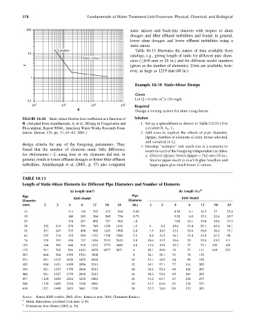
FIGURE 10.28 Static mixer friction loss coefficient as a function of Solution
R. (Adapted from Amirtharajah, A. et al., Mixing in Coagulation and 1. Set up a spreadsheet as shown in Table CD10.14 to
Flocculation, Report 90841, American Water Works Research Foun- calculate R, h L , G.
dation, Denver, CO, pp. 37, 61–63, 2001.) 2. Add rows to explore the effects of pipe diameter,
d(pipe), number of elements of static mixer selected,
and variation in Q.
design criteria for any of the foregoing parameters. They
3. Develop ‘‘scenario’’ sets (each row is a scenario) to
found that the number of elements made little difference
examine each of the foregoing independent variables:
for (#elements) > 2; using four or six elements did not, in a. Effect of d(pipe). Select d(pipe) ¼ 762 mm (30 in.).
general, result in lower effluent dosages or lower filter effluent Smaller pipes result in much higher headloss and
turbidities. Amirtharajah et al. (2001, p. 37) also compared larger pipes give much lower G values.

TABLE 10.13
Length of Static-Mixer Elements for Different Pipe Diameters and Number of Elements
a
(a) Length (mm ) (b) Length (in.) b
Pipe KMS Model Pipe KMS Model
Diameter Diameter
(mm) 2 3 4 6 12 18 24 (in.) 2 3 4 6 12 18 24
13 114 156 292 432 568 0.50 4.50 6.1 11.5 17 22.4
19 140 203 384 568 754 0.75 5.50 8.0 15.1 22.4 29.7
25 178 257 492 727 962 1.0 7.00 10.1 19.4 28.6 37.9
38 152 210 270 391 740 1108 1476 1.5 6 8.2 10.6 15.4 29.1 43.6 58.1
51 191 267 333 498 965 1429 1908 2.0 7.5 10.5 13.1 19.6 38.0 56.2 75.1
64 222 318 410 594 1153 1708 2280 2.5 8.8 12.5 16.1 23.4 45.4 67.2 90
76 270 387 498 727 1416 2115 2813 3.0 10.6 15.2 19.6 29 55.8 83.2 111
102 346 502 648 948 1832 2775 3680 4.0 13.6 19.8 25.5 37 72.1 109 145
152 511 762 994 1454 2870 4277 5671 6 20.1 30.0 39 57 113 168 223
203 664 968 1295 1924 3800 8 26.1 38.1 51 76 150
254 841 1232 1626 2435 4820 10 33.1 48.5 64 96 190
305 994 1451 1959 2896 5213 12 39.1 57.1 77 114 205
356 921 1327 1759 2648 5213 14 36.2 52.2 69 104 205
406 921 1327 1759 2648 5213 16 36.2 52.2 69 104 205
457 1124 1645 2216 3258 6483 18 44.2 64.7 87 128 255
508 1124 1645 2216 3258 6483 20 44.2 64.8 87 128 255
610 1327 1949 2623 3867 7703 24 52.2 76.8 103 152 303
Source: Kenics KMS models, 2002. (Note: Kenics is now, 2010, Chemineer-Kenics.)
a
Metric dimensions calculated from units in (b).
b
Dimensions from Kenics (2002, p. 20).