Page 318 - Fundamentals of Water Treatment Unit Processes : Physical, Chemical, and Biological

Mixing 273

Pressure differential, p (psi)
0 50 100 150 200 250 300 350
0.005
70
0.004
60
Nominal 50
0.003
Q (m 3 /s) range 40 Q (gpm)
operating
0.002
30
Nozzle:
H-15, #15280, full cone 20
0.001 Spray angle 15°
d(orifice)=9.93 mm (0.391 in.) 10
Inlet connection: 1 in.
0 0
0 50 100 150 200 250
Head (m)

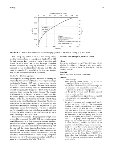
FIGURE 10.22 Flow vs. head for nozzle. (Data from Spraying Systems Co., Wheaton, IL, Catalog 70, p. B28, 2010.)
For a sharp edge orifice, C ¼ 0.611; also for any orifice, Example 10.9 Design of Jet-Mixer System
n ¼ 0.5, which conforms to value given in Catalog 70, p. B28
for their nozzles. For a nozzle, the edge is not sharp and Given
differs for each model and so the discharge coefficient Raw water is delivered to a WTP by a 1067 mm (42 in.)
must be determined by a log–log plot such as shown. The pipeline from Horsetooth Reservoir with water surface
ffiffiffiffiffi elevation 61 m (200 ft) above the plant. Let T ¼ 208C for
exponent, n, may be obtained from the same plot. The 2g
p
working purposes.
could be assimilated in a coefficient but is shown separate
here (so that more variables can be discerned). Required
Design a jet-mixer system for coagulation.
10.4.3.1.3 Design Algorithm
Solution
The design of a jet-mixing system is based first on knowing the
1. General design
relationship between flow and head, i.e., knowing the discharge
Select Spraying Systems, nozzle H-15, #15280 (as
coefficient in Equation 10.42 and=or a plot such as given in in the plot shown in Figure 10.23)
Figure 10.22 (or data from a catalog). The merit of an equation The jets have a full cone spray with cone angle 158
for the flow–head relationship is that it is amenable to use in a Let n(nozzles) ¼ 24, intended to cover the cross-
spreadsheet algorithm for design. The velocity of the jet may be sectional area of the raw-water pipeline
calculated from knowing the orifice diameter. The velocity Let the jets be oriented radial direction outward
head from the jet is dissipated as turbulence (with a portion, from a center manifold
not known, going to heat directly). The power required should Let the coagulant (alum) be injected into the manifold
flow just prior to the plane of the jet circle.
be based on the head for the nozzle (not just the velocity head,
2. Calculations
since there is a loss of head through the nozzle). The wire-to-
Set up a spreadsheet such as developed for the
water power, i.e., the power required by the pump motor, may
problem as Table CD10.12. The spreadsheet
be calculated knowing the efficiency of the pump (in its oper-
develops an algorithm to calculate for increasing
ating range) and the motor efficiency. The cost of operation manifold pressure: jet flow, jet velocity, assumed
may be obtained from the local cost of energy per kilowatt-hour pipe flow, jet flow as a fraction of raw-water flow,
(kW-h). For initial estimates a pump efficiency of 0.7 and a the power dissipated by the jet, the distance, Dz for
motor efficiency of 0.7 may be used. the intersection of the jet trajectory with the pipe
Example 10.9 enumerates a design algorithm for a jet-mixer wall, the mixing time, the hypothetical mixing vol-
system. The spreadsheet, Table CD10.12, shows for increasing ume, G, Gu, pump power imparted to water,
manifold pressure: the jet flow, jet velocity, assumed pipe flow, energy use per month (based on assumed wire-
to-water efficiency), monthly cost (based on an
jet flow as a fraction of pipe flow, the power dissipated by the
assumed cost of electric energy), and power dissi-
jet, the distance, Dz for the intersection of the jet trajectory with
pated per unit of flow (energy consumed per unit
the pipe wall, the mixing time, the hypothetical mixing vol-
of flow is about twice that calculated in Table
ume, G, Gu, pump power imparted to water, energy use per
CD10.12). Table CD10.12b shows advective tra-
month (based on assumed wire-to-water efficiency, monthly jectories for two jet flows. Figure CD10.23 is a
cost (based on an assumed cost of electric energy), and power linked plot, from trajectories restated in Table
dissipated per unit of flow (energy consumed per unit of flow is CD10.12f, showing how the trajectory is modified
about twice that calculated in Table CD10.12). by jet velocity.