Page 638 - Fundamentals of Water Treatment Unit Processes : Physical, Chemical, and Biological

Gas Transfer 593

Motor

Concrete Floor

Shaft

Impeller

D
(a) (b)

FIGURE 18.14 Turbine aeration. (a) Sketch of impeller, (b) photograph of turbine aerator basin, 1988. (Photo courtesy of S.K. Hendricks.)

still a technology that is ‘‘on-the-shelf,’’ so to speak, and is 3.0 5
still used in many situations, and partly because reviewing the D(impeller) =2.13 m
topic helps to illustrate how basic principles may be applied to
2.5
yet another kind of aeration device. 4
Figure 18.14a is a drawing of a turbine aerator with the
impeller submersed in the water of a basin. Figure 18.14b is a 2.0
photograph of an activated sludge basin with four such impel- 3
lers spaced around the basin, with two shown. Figure 18.6 W(O 2 ) (kg O 2 /kw-h) 1.5 D(impeller) =1.83 m W(O 2 ) (lb O 2 /hp-h)
shows the same scene but taken as a close-up. The basin
shown was later retrofitted, c. 1992, with fine bubble 2
diffusers. 1.0

18.3.2.2.1 General Design Requirements 0.5 1
According to Kalinske (1969a,b) the basin size must be such
that all portions of it are under the pumping influence of the
0.0 0
aerator. Sizes of surface aerators have ranged from 3 to 20 25 30 35 40 45 50 55 60
150 hp and 1–3.7 m (3–12 ft) diameter, with rotational Impeller speed (rpm)
velocities 30–60 rpm (Huang, 1975, p. 65). In general, the
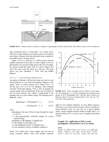
oxygen transfer rate is proportional to the rate of creation of FIGURE 18.15 Effect of impeller speed on W(O 2 ) for two impel-
new air–water interface area, which is proportional to the lers. (From Kalinske, A. A., Power consumption for oxygenation and
pumping rate for a given turbine design. The pumping rate is mixing, in W.W. Eckenfelder and J. McCabe (Eds.), Advances in
(Kalinske, 1963): Biological Waste Treatment, Pergamon Press, New York, pp. 157–
168, 1963. With permission.)

0 (18:71)
Q(pumping) ¼ k D(impeller) h v p
2
¼ k D(impeller) h v (18:72) speed for two impeller diameters. As seen, W(O 2 ) increases
0
with rpm to some peak and then declines, which is similar to a
where pump efficiency curve. As seen also, for a given impeller
Q(pumping) is the rate of flow of water through the impel- speed, a larger impeller diameter results in higher W(O 2 ). As
3
ler (m =s) noted in Section 18.3.1.2, such a curve is unique for the basin
k is the proportionality coefficient, unique for a given at hand.
0
impeller design
D(impeller) is the diameter of impeller (m)
Example 18.4 Application of W(O 2 ) versus
h is the height of rotor blades (m)
rpm(Impeller) Characteristic Curve for System
v p is the peripheral velocity of impeller (m=s)
v is the rotational velocity of impeller (radians=s) Given
3
3
Assume Q ¼ 8000 m =day (333 m =h) (or 2.1 mgd) and
3
Figure 18.15 shows how oxygen uptake mass per unit of [BOD in BOD out ] ¼ 200 mg=L (0.200 kg=m ), which
energy expended, W(O 2 ), varies with impeller rotational results in J(O 2 ) ¼ 67 kg O 2 =h. Assume also that the