Page 663 - Fundamentals of Water Treatment Unit Processes : Physical, Chemical, and Biological

618 Fundamentals of Water Treatment Unit Processes: Physical, Chemical, and Biological

ferrous metals, stainless steel, and copper, but not silver (since 1. Hydrolysis: When chlorine gas is introduced in
the silver chloride formed on contact is inert). Aqueous solu- water, dissolution occurs readily, as seen by the
tions are also corrosive. Materials used commonly for moist Henry’s law coefficient, that is, H(Cl 2 ,208C) ¼
gas and solutions include PVC, fiberglass, Kynar, polyethyl- 7283 mg=L=atm (Table H.5). Upon dissolution,
ene, certain types of rubber, Saran, Kel-F, Viton, and Teflon hydrolysis occurs with the reaction given as (Doull,
(White, 1999). 1980, p. 18)

19.3.3.2 Chlorine Demand Cl 2 þ H 2 O , HOCl þ H þ Cl (19:14)
þ
Since HOCl is a strong oxidizing agent, it reacts with a range
The HOCl further dissociates to give
of reducing substances, for example, NH 3 ,Fe ,Mn ,
2þ
2þ
NO 3 ,H 2 S, NOM, etc. (Fair et al., 1948, p. 1055). The HOCl , OCl þ H þ (19:15)

aggregate of such reactions is termed, ‘‘chlorine-demand.’’
The inorganic reactions are rapid while the NOM reactions The two species, HOCl and OCl together are des-

are, in general, slow. ignated as ‘‘free chlorine,’’ and also as ‘‘free avail-
able chlorine.’’ As evident in Equations 19.14 and
19.3.3.2.1 Breakpoint Chlorination 19.15, the distribution of the species is pH depen-
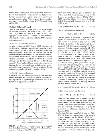
As seen by Equations 19.25 through 19.27, in subsequent dent, with the HOCl predominating at pH 7.3; for
Section 19.3.6.1, chlorine reacts with ammonia to form chlor- reference, Cl 2 is the dominant species for pH 3.3.
amines. Figure 19.4 shows a typical breakpoint chlorination Also, for reference, at pH ¼ 6.0, T ¼ 208C, HOCl
relationship caused by the reaction with ammonia. As the 0.97 fraction; and at pH ¼ 7.0, T ¼ 208C, HOCl
chlorine concentration increases the ‘‘free available chlorine’’ 0.79 fraction (Fair et al., 1948, p. 1052; White,
(the solid line) increases but at a rate less than that of ‘‘applied 1999, p. 218). The Ct’s for HOCl are generally 5–20
chlorine’’ (solid line). The difference between the ‘‘applied times higher than for OCl (see Table 19.3); in other

chlorine’’ and the ‘‘free available chlorine’’ is the ‘‘chlorine words, chlorine is the most effective at pH 7.0.
demand.’’ As the applied chlorine concentration continues to 2. Acid–base reaction equilibria for chlorine: The spe-
increase, the free available chlorine residual declines to near- cies present when chlorine gas reacts with water are
zero, which is the ‘‘breakpoint.’’ After the breakpoint, the free seen in Equations 19.14 and 19.15, that is, Cl 2 (gas),
chlorine increases linearly with the applied chlorine. Cl 2 (aq), HOCl, OCl ,Cl ,H ,OH . Thus, the first

þ

step in the analysis of acid–base equilibria is to write
19.3.3.2.2 Chlorine Reactions the reaction equations, which permit the reactant and
Chlorine in water involves a sequence of reactions. Reactions product species to be identified. Table 19.5 summar-
include hydrolysis and acid–base. In addition, chlorine acid– izes the reactions and the associated equilibrium
base equilibrium is depicted in graphical form. Finally, the equations, the latter being the second step. The reac-
formation of hypochlorites is reviewed. tions, of course, are linked. The third step is to write
the mass balance relation, that is,
C ¼ Cl 2 (aq) ¼ [HOCl] þ [OCl ] þ [Cl ] (19:16)

2.5
and the charge balance may be stated,
Chlorine applied
2.0 With the mass balance, charge balance, and five
(19:17)
[H ] ¼ [OCl ] þ [OH ] þ [Cl ]
Chlorine residual (mol Cl/mol N) 1.5 Chlorine-demand breakpoint available equilibrium equations, there are seven equations,
þ

which means that the seven unknowns may be
Free
solved. Often, the mass balance and the charge bal-
1.0
ance are combined; for example, the [Cl ] may be

chlorine
eliminated by subtracting Equation 19.17 from
Equation 19.16.
0.5
CD19.6 shows the concentrations of the aqueous
Free 3. Graphical depiction of equilibria for chlorine: Table
Chloramines chlorine chlorine species, that is, Cl 2 (aq), HOCl, OCl ,

0.0 þ
0.0 0.5 1.0 1.5 2.0 2.5 along with H ,OH ; fractions of the first three
are given also, for example, a 0 ¼ [Cl 2 ]=C(total),
Chlorine applied (mol Cl/mol N)
a 1 ¼ [HOCl]=C(total), a 2 ¼ [OCl ]=C(total), respec-

FIGURE 19.4 Illustration of breakpoint chlorination. (Adapted tively. The ancillary tables show the formulae for
from Doull, J., Drinking Water and Health, Vol. 2, National Acad- the ‘‘a’’ calculations, which are the basis for the
emy Press, Washington, DC, 1980, p. 22). calculations of the concentrations of [Cl 2 (aq)],