Page 831 - Fundamentals of Water Treatment Unit Processes : Physical, Chemical, and Biological

786 Appendix C: Miscellaneous Relations

Substituting in (C.33): 4. Mathematical relation. The functional relationship,
once DH8=R and B are found, is
DH
(C:35)
ln Y ¼
R X þ ln B DHo X
Y ¼ B e R (C:39)
which answers the often nettlesome question as to DHo X
whether to multiply or divide by 2.303. In terms of ¼ B 10 2:303 R (C:40)
the van’t Hoff equation, Equation C.35 is
DH Example C.3 Analysis of Data that Exhibit
(C:36)
ln K ¼ an Exponential Decline with Time
RT þ ln C vh
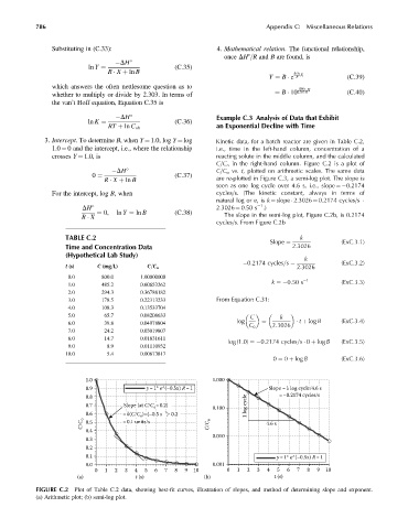
3. Intercept. To determine B, when Y ¼ 1.0, log Y ¼ log Kinetic data, for a batch reactor are given in Table C.2,
1.0 ¼ 0 and the intercept, i.e., where the relationship i.e., time in the left-hand column, concentration of a
crosses Y ¼ 1.0, is reacting solute in the middle column, and the calculated
C=C o in the right-hand column. Figure C.2 is a plot of
DH C=C o vs. t, plotted on arithmetic scales. The same data
(C:37)
0 ¼ are re-plotted in Figure C.3, a semi-log plot. The slope is
R X þ ln B
seen as one log cycle over 4.6 s, i.e., slope ¼ 0.2174
For the intercept, log B, when cycles=s. (The kinetic constant, always in terms of
natural log or e,is k ¼ slope 2.3026 ¼ 0.2174 cycles=s
1
DH 2.3026 ¼ 0.50 s .)
¼ 0, ln Y ¼ ln B (C:38) The slope in the semi-log plot, Figure C.2b, is 0.2174
R X
cycles=s. From Figure C.2b
TABLE C.2 k
(ExC:3:1)
Slope ¼
Time and Concentration Data 2:3026
(Hypothetical Lab Study)
k
(ExC:3:2)
t (s) C (mg=L) C=C o 0:2174 cycles=s ¼ 2:3026
0.0 800.0 1.00000000
k ¼ 0:50 s 1 (ExC:3:3)
1.0 485.2 0.60653262
2.0 294.3 0.36788182
3.0 178.5 0.22313233 From Equation C.31:
4.0 108.3 0.13533704
5.0 65.7 0.08208633 C k
log t þ log B (ExC:3:4)
6.0 39.8 0.04978804 ¼
C o 2:3026
7.0 24.2 0.03019807
8.0 14.7 0.01831611
log (1:0) ¼ 0:2174 cycles=s 0 þ log B (ExC:3:5)
9.0 8.9 0.01110932
10.0 5.4 0.00673817
0 ¼ 0 þ log B (ExC:3:6)

1.0 1.000
0.9 y=1* e^(–0.5x) R =1 Slope =1 log cycle/4.6 s
0.8 =–0.2174 cycles/s
0.7 Slope (at C/C =0.2) 0.100 1 log cycle
o
–1
0.6 =k(C/C )=(–0.5 s ) 0.2
·
o
C/C o 0.5 =0.1 units/s C/C o 4.6 s
0.4
0.010
0.3
0.2
0.1 y =1* e^(–0.5x) R=1
0.0 0.001
0 1 2 3 4 5 6 7 8 9 10 0 1 2 3 4 5 6 7 8 9 10
(a) t (s) (b) t (s)
FIGURE C.2 Plot of Table C.2 data, showing best-fit curves, illustration of slopes, and method of determining slope and exponent.
(a) Arithmetic plot; (b) semi-log plot.